Iterative Partial Minimization for Non-Convex Optimization: Bisection and Coordinate Descent

In Place of an Introduction

Given the nature of this publication, one feels compelled to give the reader a bit of one’s life story, so here we go.

I took Stephen Boyd’s excellent “Convex Optimization” MOOC last summer (and what with numerous references to intermediate/advanced topics in linear algebra, it was quite a challenge as far as theory was concerned, but this is not what this post is about). In one of homeworks for the course, there was a problem, in its own right, not particularly difficult or unusual. However, for this problem, I managed to come up with a solution, different from the one that was expected, which, it being something of a curiosity, I would like to share with you, my inquisitive reader.

Meet The Problem

Here is the problem formulation as given in “Additional Exercises for Convex Optimization” by Stephen Boyd and Lieven Vandenberghe (it is assigned the number 2.5 in the 2021 edition).

Let us advance towards the familiar territory by restating the problem in a more conventional (for the realm of convex optimization) mathematical form. Note that by definition \(max_{i=1,\dots,n} \lvert x_i\rvert = \left\lVert \vec{x}\right\rVert_{\infty}\), where \(\left\lVert \vec{x}\right\rVert_{\infty}\) is a so-called infinite norm for the vector \(\vec{x}=(x_1,\dots,x_n)\). Denoting a Hadamard (i.e. element-wise) product by “\(\odot\)”, we get:

A potentially confusing aspect of this notation is the use of \(a_j\), \(b_l\) for variables and \(t\), \(y\) for constants, exactly the opposite of what one would expect. The task of fitting a function to particular data means that we must find function parameters, coefficients of two polynomials in this case (hence they are the variables), that would make the function values match the given data (i.e. constants) as close as possible. Even though we will not be use this formulation, perhaps, it would be helpful to keep in mind the more conventional matrix form.

However, I found the previous notation more convenient to work with. To understand why, consider the standard form for convex/quasiconvex optimization problems:

As a standard, this is the form one typically works with when performing an analysis or implementing a solver, therefore it is advisable to transform the problem being solved into the one above, with \(f_i\) and \(h_i\) of identifiable convexity, and this is precisely what we will aim for. It should explain all the formulae “rearrangements” that follow.

The traditional approach to dealing with minimaxes (and infinite norms, in particular) consists in bounding each expression being maximized by a common new variable (we will call it \(s\)), which is then minimized. Effectively, it is a combination of two transformations:

• \(f_0(x) \rightarrow min_x \Longleftrightarrow s \rightarrow min, \mbox{s.t. }f_0(x) \le s\) (also known as an epigraph form)
• \(max_{1 \le i \le n}\; f_i(x) \le s \Longleftrightarrow \forall i = 1,\dots, n \; f_i(x) \le s\) (…)

Applying the trick, the following problem is obtained:

Taking stock of what the problem looks like at this point, one immediately notices a thing out of place - a strict inequality. Indeed, strict inequalities in constraints are problematic. For example, take a look at the simple problem below (the plot is made with Desmos).

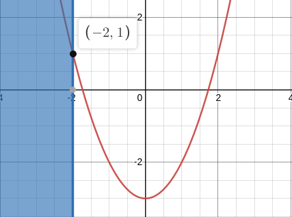
Its solution is trivial: the minimum objective value of \(1\) is attained at the boundary \(x=-2\). Now try solving a slightly modified problem.

Here, one can only talk about an optimal objective value “in the limit”. This example gets the point across rather effectively and, in doing so, justifies the lack of strict inequalities in the standard form of convex optimization problems. In relation to our problem, an inexact formulation will have to do. Following the commonly used practice, we will define a very small \(\xi\) and transform the problematic constraint into \(1 + b_1 \cdot t_i + b_2 \cdot t_i^2 \ge \xi\).

One more trivial transformation later, we get:

Looks cluttered, does it not? Just a bit? In order to make the constraint expressions more concise and easier to read, let us introduce a vector variable \(\vec{x} = (a_0, a_1, a_2, b_1, b_2)\) and rename the constants as follows: \(\vec{c_i} = (1, t_i, t_i^2, -y_i \cdot t_i, -y_i \cdot t_i^2)\), \(\vec{d_i} = (0, 0, 0, t_i, t_i^2)\).

Now, that is better!

Easily recognizable in both \(\frac{\vec{c_i}^T \cdot \vec{x} - y_i}{\vec{d_i}^T \cdot \vec{x} + 1}\) and \(\frac{(-\vec{c_i})^T \cdot \vec{x} + y_i}{\vec{d_i}^T \cdot \vec{x} + 1}\) is a linear fractional function (a fraction with affine functions in its numerator and denominator). Linear fractional functions are quasilinear, that is they are quasiconvex and quasiconcave at the same time. This fact will play an important role later on.

Remembering that our focus is on standardization, we perform the final transformation:

Unfortunately, not much can be said about \(f_i(x,s) = \frac{\vec{c_i}^T \cdot \vec{x} - y_i}{\vec{d_i}^T \cdot \vec{x} + 1} - s\) for sum of two quasiconvex functions, even if the resulting function is additively separable (i.e. \(\exists\) independent \(x\) and \(y\) s.t. \(f(x, y) = h(x) + g(y)\)), is not necessarily quasiconvex. For now it appears (if we approach the subject strictly formally and read the problem declaration as stated) it is an optimization problem in standard form with a linear objective and constraints \(f_i(x, s) \le 0\) of unidentifiable (to the extent the course has taught us) curvature. It does not fit the formal definition of (quasi-)convex optimization problem.

On this note, I am concluding the presentation and henceforth consider the problem of minimal rational fit to the exponential properly introduced.

Likewise, the problem is very pleased, I am sure.

Bisection Method

I begin by introducing the method students were expected to use. My stoic reader is invited to follow along.

The Idea Behind the Method

The previous section was concluded with the statement that the problem as given (in its last reincarnation) did not fit the definition of convex optimization problem in standard form. The said, the formal definition is purely syntactical, meaning: the fact the problem fails to satisfy this definition does not necessarily imply that it cannot be transformed into the one that does. What we are looking for is optimizing a convex function over a convex set, determined by implicit (via intersection of domains of all the functions involved) and explicit constraints, and this is exactly what we happen to have. Take a closer look at the first two constraints: \(\frac{\vec{c_i}^T \cdot \vec{x} - y_i}{\vec{d_i}^T \cdot \vec{x} + 1} \le s\) and \(\frac{(-\vec{c_i})^T \cdot \vec{x} + y_i}{\vec{d_i}^T \cdot \vec{x} + 1} \le s\). Level sets of quasiconvex functions, i.e sets \(S_{\alpha} = \{x \mid f(x) \le \alpha\}\), are, by definition of quasiconvexity, convex (for all alphas) and linear fractional functions happen to be quasiconvex. Consequently, if we treat \(s\) not as a variable, but as a constant (or a problem parameter if you will), we obtain constraints (on \(\vec{x}\)) defining convex sets.

The same applies to \(-\vec{d^T} \cdot \vec{x} - 1 \le - \xi\), but the situation is even simpler by virtue of \(-\vec{d^T} \cdot \vec{x} - 1\) being affine (i.e. convex) and \(\xi\) – a constant.

Now that \(s\) is a parameter, there is no need to minimize the objective, thus, keeping in mind that intersection of convex sets is itself convex, we have obtained a convex feasibility problem!

The general idea behind the technique can be summarized in a few sentences. Given a quasiconvex ratio function \(f(x) = \frac{p(x)}{q(x)}\) where \(p(x)\) is convex, while \(q(x)\) is concave and positive, one defines a parameterized family of functions \(\phi_t(x)\) with a non-negative parameter \(t\), such that the following holds: \(\forall x \; \phi_t(x) \le 0 \Leftrightarrow f(x) \le t\). \(\phi_t(x)\) can be constructed as follows: \(\phi_t(x) = p(x) - t \cdot q(x)\). Notice that, \(-t \cdot q(x)\) is convex, \(q(x)\) being concave and \(t\) non-negative, and, as a result, \(\phi_t(x)\) is also convex as a sum of two convex functions. Constraints in our problem fit this framework perfectly well, therefore, the technique, when applied to our problem, produces a parameterized family of convex feasibility problems:

How do we obtain a solution to the original minimization problem? The method of bisection suggests we perform a binary search over the parameter (\(s\), in our case). Given the original objective \(f_0(s) = s\), we are to find the smallest value of \(s\) for which the problem above is feasible. To this end, upper and lower limits for \(s\): \(u\) and \(l\) – must be defined. Taking into account the fact that \(s\) is itself an upper bound on the absolute value of a fit error, 0 and 1 would make safe and sound values for the lower and upper bounds respectively. If need be, we will adjust the latter after running a few experiments and determining what works in practice.

The binary search is carried out as follows: we solve the feasibility problem with \(s\) set to \(m = \frac{l+u}{2}\) and if the constraints therein turn out to be satisfiable, the optimal objective value \(s^* \in [l, m]\), otherwise it lies in the interval \((m, u]\). An iterative process is run with values of boundaries updated at each step. The stopping criterion is easily inferred for we are asked to find the solution with a certain accuracy; provided upper and lower bounds are set correctly from the start, the objective value at current iteration is always within \(u-l\) from the optimum.

Implementation

The necessary groundwork laid, it is time to get down to coding. I will use cvxpy for the purpose. Where no random number generation was involved, I found that it worked just as well as matlab for all the problems in the course. Here is the version I was using:

1
2
:~$ pip3 list | grep cvxpy
cvxpy                  1.1.18

The entire source code for the minimax rational fit to the exponential problem can be found here; therein classes relevant at this time are FitProblem (functionality common to both bisection and my method) and BisectionFitProblem.

Let us begin with the simplest task of all – generating the data (i.e. constants).

1
2
3
4
5
6
7
8
9
10
11
12
13
14
15
16
17
18
def define_domain_bounds(self):
    self.k = 201
    self.lb = -3
    self.ub = 3

def function_to_fit(self, x):
    return np.exp(x)

def generate_data(self):

    self.define_domain_bounds()

    self.t = np.array([ self.lb + (self.ub - self.lb) * i / (self.k - 1.0) 
        for i in range(self.k) ])

    self.tsq = np.multiply(self.t, self.t)

    self.y = self.function_to_fit(self.t)

There is nothing to tell in the way of commentary for this code pretty much follows the problem statement. Now let us declare the variables.

1
2
3
4
5
6
7
8
9
10
11
12
def declare_variables_and_parameters(self):

    self.a0 = cp.Variable()
    self.a1 = cp.Variable()
    self.a2 = cp.Variable()

    self.b1 = cp.Variable()
    self.b2 = cp.Variable()

    self.z = cp.Variable(self.k, pos = True)
    
    self.s = cp.Parameter()

For the sake of readability by future self (and other people, too), I decided to keep the original coefficients: \(a_0\), \(a_1\), \(a_2\), \(b_1\), and \(b_2\); after all, vector variable \(\vec{x}\) was only introduced in order to simplify the discussion. As to \(s\), it is declared as a parameter which would allow us to adjust its value without recompiling the problem each time.

So the final (at least, as far as implementation of bisection goes) variant of the problem we have set out to work on is:

Variable z requires an explanation. Perhaps, the reader remembers a trick with substituting a very small \(\xi\) for 0 aiming to circumvent the “no strict inequalities” rule. I have some news about it, as per tradition, good and bad. The good news is, formally speaking, we do not really need it: cvxpy offers pos attribute one can set to True for a variable, thereby demanding it to be positive. This is exactly what we will do, adding \(1 + b_1 \cdot t_i + b_2 \cdot t_i^2 = z_i\) constraints along the way. The bad news is that, at present, setting this attribute does not seem to accomplish anything. Take a look at cvxpy implementation

1
2
if var.is_pos() or var.is_nonneg():
    constr.append(obj >= 0)

Evidently, pos and nonneg attributes are processed in exactly the same fashion (unless I am missing something), our only consolation being that all the calculations are approximate and getting an exact zero is fairly unlikely. Thus we leave the declarations as is: at the very least, it will look perfectly correct “on our end”.

Declaring constraints consists in essentially a one-to-one conversion from mathematical notation to code.

1
2
3
4
5
6
7
8
9
10
11
def declare_constraints(self):

    self.constraints = [ np.ones(self.k) + self.b1 * self.t + 
        self.b2 * self.tsq == self.z ]
    #[...]
    self.constraints.extend(
    	[ self.a0 + self.a1 * self.t + self.a2 * self.tsq - 
    	    cp.multiply(self.y, self.z) <= self.z * self.s, 
    	  self.a0 + self.a1 * self.t + self.a2 * self.tsq - 
    	    cp.multiply(self.y, self.z) >= -self.z * self.s,
    	])

All the constraints having transcended into their programmatic being, there remains an objective only…

1
2
def declare_objective(self):
	self.objective = cp.Minimize(0)

A constant objective signifies that it is a feasibility problem.

Now that we are done with the declarations, let us proceed by implementing the imperative part, bisection, that would allow us to compute the optimal solution by solving a series of feasibility problems.

1
2
3
4
5
6
7
8
9
10
11
12
13
14
15
16
17
18
19
20
21
22
23
24
25
def solve(self, u):

    time = 0.0
    steps = 0
    l = 0.0

    while u - l > self.eps:

        self.s.value = (u + l) / 2.0

        self.call_solver() 

        time += self.prob.solver_stats.solve_time
        steps += 1

        if self.prob.status == 'optimal':
            u = self.s.value
        else:
            l = self.s.value

        self.s.value = u
        self.call_solver()
        assert(self.prob.status == 'optimal')

        return (steps, time)

Bookkeeping functionality aside, this is a straightforward implementation of binary search and, for this reason, there should be no difficulty in understanding it. Especially if one realizes that throughout execution of Solve(), the following invariant is maintained: the problem is always feasible with \(s\) set to the current upper bound \(u\), whereas \(s\) equal to the lower bound \(l\) may or may not satisfy the constraints. This remark should explain the last call to a solver: it finds the best (to the degree permitted by the accuracy \(\epsilon\)) values for \(a_0\), \(a_1\), \(a_2\), \(b_1\), \(b_2\) variables by setting \(s\) in such a way that the solution is guaranteed to exist.

One might find the line self.call_solver() somewhat furtive. Indeed, which solver should we choose?

As it has been mentioned already, treating \(s\) as a parameter rather than a variable left us with a series of convex optimization problems. In this particular case the situation is even better – not only are the constraints convex, they are linear (or rather, affine, if one must maintain an air of punctiliousness about them) in all the variables: \(a_0\), \(a_1\), \(a_2\), \(b_1\), \(b_2\), and \(\vec{z}\)! The fact that all the expressions used in declare_constraints() are affine can easily be checked by examining the entries we put into the constraints array; however, the idea of making sure cvxpy also classifies them as such seems a capital one.

1
2
3
4
5
6
7
8
9
10
11
12
13
class FitProblem:
    #[...]
    def print_curvature(self):
        print("Objective's curvature:", self.objective.expr.curvature)
        for i in range(len(self.constraints)):
            print("Curvature of constraint", i + 1,":", 
                self.constraints[i].expr.curvature)

class BisectionFitProblem(FitProblem): #[...]

bp = BisectionFitProblem()
bp.create_problem()
bp.print_curvature()

This script will produce the output below:

1
2
3
4
Objective's curvature: CONSTANT
Curvature of constraint 1 : AFFINE
Curvature of constraint 2 : AFFINE
Curvature of constraint 3 : AFFINE

Feasibility problems with affine constraints belong to the linear programs (LP) category (historically, optimization problems of certain classes, when written down in symbolic form, have been called “programs” so I will use the terms interchengeably), hence, theoretically, we could employ an LP solver for the task. For instance, a staple of optimization methods-related scholastic pursuits, the simplex method, should do the job. However, practice sometimes fails to meet theory. Attempting to use SCIPY solver that came with the cvxpy brought no joy: it turned out, their simplex method implementation did not support constraint specification in matrix form and the amount of effort put into expanding matrix equasions row by row would have been hard to justify. Other methods (interior point, for example) ran into numerical issues on some iterations of binary search. I could try and get to the bottom of the problem, but it was not worth it: on the iterations where SCIPY showed no issues, ECOS still run much faster. So I decided to go with the latter.

1
2
def call_solver(self):
    self.prob.solve(solver = cp.ECOS)

cvxpy and ECOS Interaction: an Inside Look

Embedded Conic Solver (ECOS) accepts convex second-order cone programs of the type:

This piculiar-looking inequality \(\le_\mathcal{K}\) goes by the name of generalized inequality with respect to a (proper convex) cone \(\mathcal{K}\). By definition,

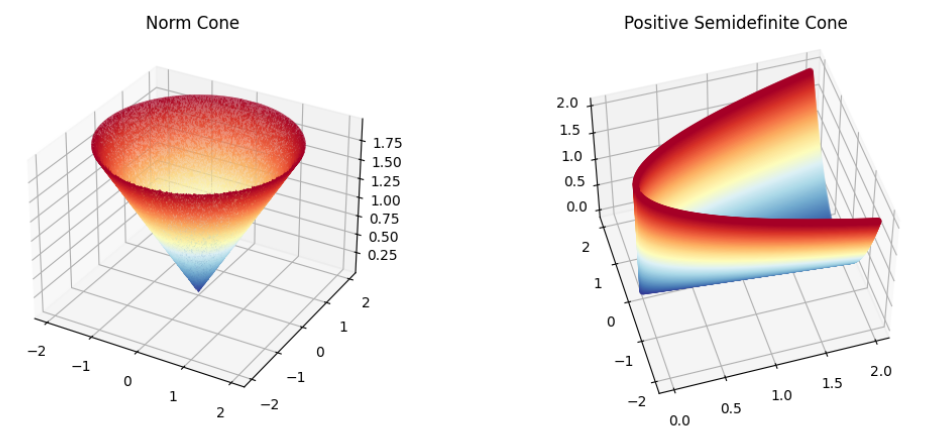
Taking the cone \(\mathcal{K}\) to be a positive orthant \(\mathbb{R}_+^n\) (a generalization of the notion of positive quadrant to \(n\) dimensions), one obtains regular linear inequalities, the problem thereby reducing to an LP.

Whether it is in any way condusive to progress on the task at hand is up for debate, but, with all probability, the most curious of the readers would like to know how the problems are represented and processed internally (by cvxpy). Let us all succumb to the temptation and peer inside. Along the way, we will also make sure that ECOS, indeed, solves a linear program.

A good place to start an investiagtion is a call to Problem.solve() with verbose flag set to True. Careful inspection of whatever appears on the console informs us that cvxpy has identified our program as following their DCP (Disciplined Conic Program) rules (adhering to the rules guarantees that the curvature of all the constraints in the problem is known) and suitable for solving with ECOS; but before being handed over to a solver, the program must undergo the transformation:

1
Dcp2Cone -> CvxAttr2Constr -> ConeMatrixStuffing -> ECOS 

According to the documentation, Dcp2Cone reduction “takes as input (minimization) DCP problems and converts them into problems with affine objectives and conic constraints whose arguments are affine.” In the process, Dcp2Cone() calls CvxAttr2Constr(), where the attributes found in variable declarations (pos in our case) are handled, followed by ConeMatrixStuffing() that constructs \(\vec{c}, A, \vec{b}, G, \vec{h}\) - matrices and vectors to be passed to ECOS, and concluded by ECOS() that invokes its namesake solver. Why not take a closer look at the last call?

1
2
3
4
solution = ecos.solve(data[s.C], data[s.G], data[s.H],
    cones, data[s.A], data[s.B],
    verbose=verbose,
    **solver_opts)

Observe that the matrix names are the same as those used for the ECOS problem statement in mathematical notation, which, of course, is not a coincidence.

After exploring cvxpy source code for a little while, I managed to find a quick way of extracting the matrices passed to ECOS. For convenience, let us temporarily reduce the number of data points from 201 to 11,

1
2
3
4
def define_domain_bounds(self):
    self.k = 11
    self.lb = -3
    self.ub = 3

adjust output settings, and create an instance of bisection problem to experiment with.

1
2
3
4
5
6
7
8
9
10
11
12
import sys
import numpy as np
from minimax_fit import * #our impelementation of minimax fit to the exponential

#the printing options that produce readable matrices
np.set_printoptions(threshold = sys.maxsize)
np.set_printoptions(precision = 2)
np.set_printoptions(suppress = True) 

p = BisectionFitProblem()
p.create_problem()
data = p.prob.get_problem_data(cp.ECOS)

Now we are all set to do the digging.

Coefficients of the linear objective function must all be zero since it is a feasibility problem.

1
2
>>> data[0]['c']
array([0., 0., 0., 0., 0., 0., 0., 0., 0., 0., 0., 0., 0., 0., 0., 0.])

Indeed, they are! Now let us examine the constraints.

1
2
3
4
5
6
7
8
9
10
11
12
13
14
15
>>> print(data[0]['A'].todense())
[[-1.   0.   0.   0.   0.   0.   0.   0.   0.   0.   0.  -3.   9.   0.    0.   0. ]
[ 0.  -1.   0.   0.   0.   0.   0.   0.   0.   0.   0.  -2.4  5.8  0.   0.   0. ]
[ 0.   0.  -1.   0.   0.   0.   0.   0.   0.   0.   0.  -1.8  3.2  0.   0.   0. ]
[ 0.   0.   0.  -1.   0.   0.   0.   0.   0.   0.   0.  -1.2  1.4  0.   0.   0. ]
[ 0.   0.   0.   0.  -1.   0.   0.   0.   0.   0.   0.  -0.6  0.4  0.   0.   0. ]
[ 0.   0.   0.   0.   0.  -1.   0.   0.   0.   0.   0.   0.   0.   0.   0.   0. ]
[ 0.   0.   0.   0.   0.   0.  -1.   0.   0.   0.   0.   0.6  0.4  0.   0.   0. ]
[ 0.   0.   0.   0.   0.   0.   0.  -1.   0.   0.   0.   1.2  1.4  0.   0.   0. ]
[ 0.   0.   0.   0.   0.   0.   0.   0.  -1.   0.   0.   1.8  3.2  0.   0.   0. ]
[ 0.   0.   0.   0.   0.   0.   0.   0.   0.  -1.   0.   2.4  5.8  0.   0.   0. ]
[ 0.   0.   0.   0.   0.   0.   0.   0.   0.   0.  -1.   3.   9.   0.   0.   0. ]]

>>> print(data[0]['b'])
[-1. -1. -1. -1. -1. -1. -1. -1. -1. -1. -1.]

Note that the generated matrices contain enough zeros to deem them sparse, so cvxpy, reasonably, uses appropriate data structure from numpy to store the constraint coefficients for equalities and inequalities and pass them to ECOS, who, working in conglomerate, also understands sparse matrices. On our end, the matrices must be transfomed back into dense ones before printing.

Interpreting \(A\) and \(b\) should not be a challenge. I think, one will find that setting vector of variables to \(\vec{x} = (z_1, \dots, z_k, b_1, b_2, a_0, a_1, a_2)\) translates the constraint \(\vec{1} + b_1 \cdot \vec{t} + b_2 \cdot \vec{t} \odot \vec{t} = \vec{z}\) (or equivalently, \(-\vec{z} + b_1 \cdot \vec{t} + b_2 \cdot \vec{t} \odot \vec{t} = -\vec{1}\)) into its matrix form \(A \cdot \vec{x} = \vec{b}\) with \(A\) specified above.

Now let us inspect the inequalities-related matrices.

1
2
3
4
5
6
7
8
9
10
11
12
13
14
15
16
17
18
19
20
21
22
23
24
25
26
27
28
29
30
31
32
33
34
35
36
37
38
39
>>> print(data[0]['G'].todense())
[[ -1.    0.    0.    0.    0.    0.    0.    0.    0.    0.    0.    0.   0.    0.    0.    0. ]
[  0.   -1.    0.    0.    0.    0.    0.    0.    0.    0.    0.    0.   0.    0.    0.    0. ]
[  0.    0.   -1.    0.    0.    0.    0.    0.    0.    0.    0.    0.   0.    0.    0.    0. ]
[  0.    0.    0.   -1.    0.    0.    0.    0.    0.    0.    0.    0.   0.    0.    0.    0. ]
[  0.    0.    0.    0.   -1.    0.    0.    0.    0.    0.    0.    0.   0.    0.    0.    0. ]
[  0.    0.    0.    0.    0.   -1.    0.    0.    0.    0.    0.    0.   0.    0.    0.    0. ]
[  0.    0.    0.    0.    0.    0.   -1.    0.    0.    0.    0.    0.   0.    0.    0.    0. ]
[  0.    0.    0.    0.    0.    0.    0.   -1.    0.    0.    0.    0.   0.    0.    0.    0. ]
[  0.    0.    0.    0.    0.    0.    0.    0.   -1.    0.    0.    0.   0.    0.    0.    0. ]
[  0.    0.    0.    0.    0.    0.    0.    0.    0.   -1.    0.    0.   0.    0.    0.    0. ]
[  0.    0.    0.    0.    0.    0.    0.    0.    0.    0.   -1.    0.   0.    0.    0.    0. ]

[ -0.5   0.    0.    0.    0.    0.    0.    0.    0.    0.    0.    0.   0.    1.   -3.    9. ]
[  0.   -0.6   0.    0.    0.    0.    0.    0.    0.    0.    0.    0.   0.    1.   -2.4   5.8]
[  0.    0.   -0.7   0.    0.    0.    0.    0.    0.    0.    0.    0.   0.    1.   -1.8   3.2]
[  0.    0.    0.   -0.8   0.    0.    0.    0.    0.    0.    0.    0.   0.    1.   -1.2   1.4]
[  0.    0.    0.    0.   -1.    0.    0.    0.    0.    0.    0.    0.   0.    1.   -0.6   0.4]
[  0.    0.    0.    0.    0.   -1.5   0.    0.    0.    0.    0.    0.   0.    1.    0.    0. ]
[  0.    0.    0.    0.    0.    0.   -2.3   0.    0.    0.    0.    0.   0.    1.    0.6   0.4]
[  0.    0.    0.    0.    0.    0.    0.   -3.8   0.    0.    0.    0.   0.    1.    1.2   1.4]
[  0.    0.    0.    0.    0.    0.    0.    0.   -6.5   0.    0.    0.   0.    1.    1.8   3.2]
[  0.    0.    0.    0.    0.    0.    0.    0.    0.  -11.5   0.    0.   0.    1.    2.4   5.8]
[  0.    0.    0.    0.    0.    0.    0.    0.    0.    0.  -20.6   0.   0.    1.    3.    9. ]

[ -0.5   0.    0.    0.    0.    0.    0.    0.    0.    0.    0.    0.   0.   -1.    3.   -9. ]
[  0.   -0.4   0.    0.    0.    0.    0.    0.    0.    0.    0.    0.   0.   -1.    2.4  -5.8]
[  0.    0.   -0.3   0.    0.    0.    0.    0.    0.    0.    0.    0.   0.   -1.    1.8  -3.2]
[  0.    0.    0.   -0.2   0.    0.    0.    0.    0.    0.    0.    0.   0.   -1.    1.2  -1.4]
[  0.    0.    0.    0.    0.    0.    0.    0.    0.    0.    0.    0.   0.   -1.    0.6  -0.4]
[  0.    0.    0.    0.    0.    0.5   0.    0.    0.    0.    0.    0.   0.   -1.    0.    0. ]
[  0.    0.    0.    0.    0.    0.    1.3   0.    0.    0.    0.    0.   0.   -1.   -0.6  -0.4]
[  0.    0.    0.    0.    0.    0.    0.    2.8   0.    0.    0.    0.  0.   -1.   -1.2  -1.4]
[  0.    0.    0.    0.    0.    0.    0.    0.    5.5   0.    0.    0.  0.   -1.   -1.8  -3.2]
[  0.    0.    0.    0.    0.    0.    0.    0.    0.   10.5   0.    0.  0.   -1.   -2.4  -5.8]
[  0.    0.    0.    0.    0.    0.    0.    0.    0.    0.   19.6   0.  0.   -1.   -3.   -9. ]]

>>> print(data[0]['h'])
[0. 0. 0. 0. 0. 0. 0. 0. 0. 0. 0. 0. 0. 0. 0. 0. 0. 0. 0. 0. 0. 0. 0. 0. 0. 0. 0. 0. 0. 0. 0. 0. 0.]

A little deliberation will convince the reader that, from \(G \cdot \vec{x} \preceq h\), the original constraints are recoverable as:

• \(\vec{z} \succ \vec{0}\), transformed into \(-\vec{z} \preceq \vec{0}\)
• \(\frac{ a_0 + a_1 \cdot \vec{t} + a_2 \cdot \vec{t} \odot \vec{t}}{\vec{z}} - \vec{y} \le s \cdot \vec{1}\), equivalent to \(-\vec{z} \odot (\vec{y} + s \cdot \vec{1}) + a_0 + a_1 \cdot \vec{t} + a_2 \cdot \vec{t} \odot \vec{t} \preceq \vec{0}\)
• \(\frac{a_0 + a_1 \cdot \vec{t} + a_2 \cdot \vec{t} \odot \vec{t}}{\vec{z}} - \vec{y} \ge -s \cdot \vec{1}\), equivalent to \(\vec{z} \odot (\vec{y} - s \cdot \vec{1}) - a_0 - a_1 \cdot \vec{t} - a_2 \cdot \vec{t} \odot \vec{t} \preceq \vec{0}\)

All that remains to be done now is making sure that the inequalities are taken with relation to the right cone.

1
2
>>> data[0]['dims']
(zero: 11, nonneg: 33, exp: 0, soc: [], psd: [], p3d: [])

It turns out, cvxpy uses two cones: one consisting of a single point \((0,\dots,0)\) in 11-dimensional space (which is there to facilitate the equality constraints: \(\vec{1} + b_1 \cdot \vec{t} + b_2 \cdot \vec{t} \odot \vec{t} - \vec{z} \in \{(0,\dots,0)\}\)) and another one, a positive orthant in 33-dimentional space (for the 33 ineqialities we have just deduced). Cones of all other types are set to 0 dimensions as they should (leading to conclusion that ECOS, in fact, receives an instance of a linear program).

I hope the reader enjoyed this brief tour of “under the hood”. Now back to the task at hand!

Assesment

Let us see how well (if at all) our implementation works.

1
2
3
4
5
6
bp = BisectionFitProblem()
bp.create_problem()
bp_steps, bp_time = bp.solve(1)
print("Bisection method took", "{0:0.3f}".format(bp_steps), "iterations and",
    bp_time, "ms to solve the problem")
print("Attained objective value is", bp.evaluate_objective())

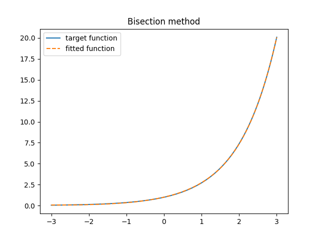
Executing this tiny script produces the output below:

1
2
Bisection method took 10 iterations and 0.027 ms to solve the problem
Attained objective value is 0.023317278116957378

Well, bisection finds a solution to the accuracy requested in a reasonable amount of time while taking a modest number of steps. The issue with this method is numerical instability. For starters, it is sensitive to the initial value of the parameter \(s\); for example, even though the optimal value ends up being significantly less than 0.1, setting \(u\) to 0.1 results in an exception.

Likewise, an attempt to solve the same program, but with a higher accuracy, leads to the same unfortunate outcome. Of course, one can tackle the issue by adjusting solver’s parameters, for example, like this:

1
2
3
4
5
6
7
8
9
10
11
12
13
class BisectionFitProblemHighEps(BisectionFitProblem):
"""Bisection method with higher accuracy"""

    def __init__(self):
        self.eps = 0.0001 #eps: 0.001 -> 0.0001

    def call_solver(self):
        solver = cp.ECOS
        try:
            self.prob.solve(solver = solver)
        except:
            #default abstol = 1.0e-7
            self.prob.solve(solver = solver, abstol = 1.0e-3)

Although this approach does allow to compute the solution with a higher accuracy (i.e. smaller \(\epsilon\)) in this particular case, it is a tough balancing act in general. Let me explain why.

At heart of the ECOS solver algorithm is a fancy variant of interior point method the authors describe as “a standard primal-dual Mehrotra predictor-corrector interior-point method with self-dual embedding”. Consider a typical feasibility problem ECOS is designed for, but with inequalities relative to the ordinary positive orthant (no sophisticated cones); minimax rational fit to the exponential happens to be of this kind. It can be transformed into an optimization problem with an extra variable \(u\) (if the optimal value of \(u\) turns out to be positive, the original problem is infeasible).

To tackle this problem (let us call it a “main problem”), classical interior point method would iteratively solve a series of sub-problems:

for an increasing parameter \(t\), following a so-called central path. Solution to this problem for a particular \(t\) gives us feasible (but not necessarily optimal) points for the main primal problem and its dual. As \(t\) goes to infinity, points on the central path approach optimal solution to the main problem and, therefore, the duality gap, a gap between primal and dual objectives, vanishes. It is now clear why the length of duality gap can be (and is!) used as a stopping criterion. ECOS’s abstol parameter sets “absolute tolerance on the duality gap”. By increasing it, we are terminating the algorithm earlier and thus potentially reducing the accuracy, the very thing we have set out to increase!

All the numerical issues aside, bisection method computes a pretty good-looking fit. Check it out!

Where the Inspiration Comes from

The bisection method presented above was the expected way of solving quasiconvex problems and the minimax rational fit to the exponential, in particular. To this end, it was helpfully explained to us during a lecture. However, this is not how I arrived at the solution submitted as a part of that homework. The rationale behind it was that I encountered bisection once only (in the recent years), whereas of coordinate ascent/descent and expectation maximization algorithms, I heard so many times – I lost count. In fact, one will be hard pressed to find a reasonably comprehensive machine learning course where the subject would not have come up.

Here is a quick recap of the relevant material.

Consider K-means clustering. Given \(n\) points in \(\mathbb{R}^d\): \(\vec{x_1} \in \mathbb{R}^d, \dots, \vec{x_n} \in \mathbb{R}^d\), the task is to partition them in \(K\) clusters with proximity of two points determined by Euclidean distance between them. It can be restated as an optimization problem:

where \(c_i \in \{1,\dots,K\} \; (i = 1,\dots,n)\) assigns \(i^{th}\) point to its cluster and each of \(\vec{\mu_i} \in \mathbb{R}^d \; (i=1,\dots,K)\) is a cluster centroid. A collection of vectors \(\vec{\mu_i}\), stacked horizontally, form a matrix: \(M = [\vec{\mu_1}, \dots, \vec{\mu_K}] \subseteq \mathbb{R}^{d \times K}\).

This objective is neither convex nor continuous (the indicator function spoiling all the fun) and, as such, does not admit of methods from the convex optimization toolbox. Another approach is needed. Notice that, given a particular value of \(\vec{c}\), the objective becomes a sum of norms, i.e. a convex function, and this is the feature leveraged by K-means.

Underlying K-means is a coordinate ascent/descent algorithm. In general terms, the algorithm consists in maximizing/minimizing over a (proper) subset of coordinates of a vector variable while remaining coordinates remain fixed; it is performed in an iterative manner alternating which subset is “fixed” at each step. For K-means, the vector variable is \((c_1,\dots,c_n,\mu_1^{(0)},\dots,\mu_1^{(d)},\dots,\mu_K^{(0)},\dots,\mu_K^{(d)})\) and its coordinates are partitioned into \(M\) and \(\vec{c}\). Multiple iterations are necessary because \(M\) and \(\vec{c}\) are not independent.

Below is a sketch of K-means algorithm.

• Initialize \(M\) with a set of random vectors
• Iterate
  • Step 1: For fixed \(M\):
  \[c_i = \argmin_{k \in \{1,\dots, K\} } \left\lVert\vec{x_i} - \vec{\mu_k}\right\rVert^2_2 \mbox{ (computed in a loop over k)}\]
  • Step 2: For fixed \(\vec{c}\):
  \[\vec{\mu_k} = \argmin_{\vec{\mu_k}} \sum_{i:\; c_i = k} \left\lVert\vec{x_i} - \vec{\mu_k}\right\rVert^2_2 = \frac{1}{n_k} \cdot \sum_{i:\; c_i = k} x_i\]
• Until \(M\) and \(\vec{c}\) stop changing

A variant of coordinate ascent is used in probabilistic setting. Given are \(n\) data points \(X = \{x_1,\dots,x_n\}\) drawn independently from a probability distribution \(p(x \mid \vec{\theta})\), that is \(x_i \stackrel{iid}{\sim} p(x\mid\vec{\theta})\), where \(\vec{\theta}\) encompasses distribution parameters. For example, for a Gaussian distribution with mean \(\mu\) and standard deviation \(\sigma\), \(\vec{\theta} = (\mu, \sigma)\). One would like to find such values of parameters \(\vec{\theta}\) that would maximize the probability of generating the observed data. This is where the notion of likelihood comes is handy. Probability density (or, for discrete variables, probability mass function), viewed as a function of distribution parameters for the given data sample, is referred to as a likelihood of data given the model parameters. Recalling that the data points are independent, the likelihood is computed in this way:

The task is to find \(\vec{\theta}\) maximizing \(\mathcal{L}(\vec{\theta})\).

For convenience, log-likelihood (\(log \mathcal{L}(\vec{\theta}) = l(\vec{\theta})\)) is often used instead; \(log(x)\) being a nondecreasing function, it does not change the outcome:

When the probability density is log-concave in parameters \(\vec{\theta}\), one may enjoy a convex optimization problem with nice properties like any local maximum being a global one. Some even admit of an analytical solution (for example, \(x_i \stackrel{iid}{\sim} \mathcal{N}(x\mid\mu, \sigma)\)). Other times, however, maximizing over \(\vec{\theta}\) is tricky, but if we divide the distribution parameters \(\vec{\theta} = [\vec{\theta}_1, \vec{\theta}_2]\) into two groups, it might be easy to compute \(\vec{\theta}_{1, ML} = \argmax_{\vec{\theta}_1} l(\vec{\theta}_1 \mid \vec{\theta}_2)\) and \(\vec{\theta}_{2, ML} = \argmax_{\vec{\theta}_2} l(\vec{\theta}_2 \mid \vec{\theta}_1)\). As my perceptive reader will, no doubt, have guessed, the coordinate ascent algorithm alternates between steps 1 and 2, maximizing log-likelihood over \(\vec{\theta}_{\langle step \rangle}\) while keeping \(\vec{\theta}_{\langle 3 - step \rangle}\) fixed.

The ubiquitously renowned expectation maximization (EM) algorithm takes the similar approach with two alternating optimization steps. We are in the same probabilistic setting, but imagine that now, in addition to the observed data \(X\), there are also latent variables \(z_i\), \(i = 1, \dots, m\), values of which are unknown.

The task is to maximize the likelihood of the marginal distribution: \(p(x_1,\dots,x_n\mid\theta) = \idotsint p(x_1,\dots,x_n, z_1,\dots,z_m\mid\theta) \,dz_1 \dots dz_m = \int p(X, Z\mid\theta) \,dZ\) \(\left( p(x_1,\dots,x_n\mid\theta) = \sum_{z_1}\cdots\sum_{z_m}p(x_1,\dots,x_n, z_1,\dots,z_m\mid\theta) = \sum_{Z} p(X, Z\mid\theta)\right)\) \((\mbox{ for discrete distributions})\)

Before continuing, please, take a note of the switch to discussion in terms of joint distributions \(p(X)\) and \(p(X, Z)\). Now the product/summation over data points is gone. There is still an integration over variables \(z_i\) (to compute a marginal distribution), but it is of different origin.

A few relatively straightforward formula manipulations will produce the following expression for the log-likelihood:

where \(q(Z)\) is an arbitrary distribution (that makes \(l()\) a high-order function or a functional).

Writing down the likelihood in this form makes it possible to construct the expectation maximization algorithm:

• Initialize \(\theta\) with a random value (vector or scalar, depending on the dimensionality of distribution parameters)
• Iterate
  • Step 1: For fixed \(\theta\):
  \[q(Z)_{ML} = \argmax_q l(q \mid \theta)\]

        Take a closer look at the second summation term in the expression for \(l(\theta, q)\) above. One can easily recognize Kullback–Leibler divergence between \(q(Z)\) and \(p(Z\mid X,\theta)\), which is always positive except for when \(q(Z) = p(Z\mid X,\theta)\). It gives us the solution:

  \[q(Z)_{ML} = p(Z\mid X,\theta)\]
  • Step 2: For fixed \(q(Z)\):
  \[\theta_{ML} = \argmax_{\theta} l(\theta \mid q)\]

        Notice that in case of \(q(Z) = p(Z\mid X,\theta)\)

  \[l(\theta) = \int p(Z\mid X,\theta) \cdot log p(X,Z\mid\theta) \,dZ - \int p(Z\mid X,\theta) \cdot log p(Z\mid X,\theta) \,dZ =\] \[E_{Z}[log p(X,Z\mid\theta)\mid X] - H(p)\]

        Therefore,

  \[\theta_{ML} = \argmax_{\theta} E_{Z}[log p(X,Z\mid\theta)\mid X]\]

        which, wherever EM is applicable, is much easier to compute than the original problem.

• Until \(l(\theta, q)\) converges

This approach turns up in many settings: K-means and K-medoids, mixture models and soft clustering, learning models from incomplete data, probabilistic matrix factorization, just to name a few. No wonder, it is the first technique that comes to mind.

I realize it was too terse a discussion to be of great educational value; the intention was to give an intuition for the method and show where my solution stemmed from. So where does one find information to develop in-depth understanding of EM and other coordinate ascent/descent - based algorithms? The simple answer is: just about everywhere, but who can resist singling out favorites? Mine, sources where the level of comprehensiveness of the subject treatment is exactly to my liking, are the course on Machine Learning from Columbia University taught by John Paisley and “Pattern Recognition and Machine Learning” by Christopher Bishop. By the way, these are the sources I consulted while writing this section.

Coordinate Descent Method

Having learnt the founding principles, let us apply them to the minimax rational fit to the exponential problem. Hop in!

I begin by reminding the reader what the problem in question was.

Simple algebraic manipulations will give us:

Upon cursory inspection, terms \(s \cdot b_1\) and \(s \cdot b_2\) are an obvious complication for they make the constraints non-convex, whereas all other summation terms are linear in the variables. The solution in line with what we have just learnt would be to partition the variables involved in nonlinear terms into two sets and perform partial minimization over one set while keeping the other one constant. The two disjoint sets would be \(\{b_1, b_2\}\) and \(\{s\}\); as for \(a_0, a_1, a_2\), we can leave them as variables in both steps.

As a result, we are left with two linear programs. Let us code them up! In my python script, the relevant class is CoordinateDescentFitProblem.

1
2
3
4
5
6
7
8
9
10
11
12
13
class CoordinateDescentFitProblem(FitProblem):
    #[...]
    def declare_variables_and_parameters(self):

        #base class takes care of a0, a1, a2, b1, b2, and z
        super().define_variables_and_parameters()

        #problem 1
        self.s_p = cp.Parameter()    

        #problem 2
        self.s = cp.Variable(nonneg = True)
        self.z_p = cp.Parameter(self.k)

On the one hand, variables \(b_1\) and \(b_2\) appear in one expression only: \(z_i = 1 + b_1 \cdot t_i + b_2 \cdot t_i^2\); on the other hand, expression involving \(z\) contains no variables other than \(b_1\), \(b_2\) and \(z\) itself, therefore, for the second problem (where \(b_1\) and \(b_2\) are constant), a single parameter, \(\vec{z_p}\), would suffice.

1
2
3
4
5
6
7
8
9
10
11
12
13
14
15
16
17
18
19
20
21
22
23
24
25
26
def declare_objective(self):

    #objective for the first problem:
    self.objective = cp.Minimize(0)
    
    #objective for the seond problem:
    self.objective2 = cp.Minimize(self.s) 

def declare_constraints(self):

   #constraints for the first problem:
   self.constraints = [ 
       np.ones(self.k) + self.b1 * self.t + self.b2 * self.tsq == self.z,
       self.a0 + self.a1 * self.t + self.a2 * self.tsq - 
           cp.multiply(self.y, self.z) <= self.s_p * self.z, 
       self.a0 + self.a1 * self.t + self.a2 * self.tsq - 
           cp.multiply(self.y, self.z) >= -self.s_p * self.z
   ])
   
   #constraints for the second problem:
   self.constraints2 = [ 
       self.a0 + self.a1 * self.t + self.a2 * self.tsq - 
           cp.multiply(self.y, self.z_p) <= self.s * self.z_p,
       self.a0 + self.a1 * self.t + self.a2 * self.tsq - 
           cp.multiply(self.y, self.z_p) >= -self.s * self.z_p
   ]

With \(s\) “demoted” to a parameter, the first descent step turns into a feasibility problem that determines whether it is possible to find such values of \(\vec{a}\) and \(\vec{b}\) that would satisfy the threshold on the fit error specified by \(s\).

The constraints look pretty much identical in both linear programs with the exception for the absent condition on \(z\) in the second one, where \(z\) is constant.

A small hindrance must be addressed before we can implement the solve() method. We are asked to find an optimal objective value with a certain accuracy. For bisection method, it was easy to do – the algorithm maintained an interval of decreasing length an optimal value of the objective belonged to. Here, we are deprived of such luxuries. Coordinate descent terminates as soon as objective converges, i.e. (nearly) stops changing, which, in practical terms, translates into two consecutive objective values being within a small distance \(\epsilon\) from each other. The only thing we can do is to set \(\epsilon\) very small and compute the objective as precise as possible hoping the resulting accuracy will be at least as good as the one requested. Here we go.

1
2
def __init__(self):
    self.eps = 0.0000001

The declaration part done and dusted, I present the coordinate descent itself.

1
2
3
4
5
6
7
8
9
10
11
12
13
14
15
16
17
18
19
20
21
22
23
24
25
26
27
28
29
30
31
32
33
def solve(self, sv):

    val = np.finfo(float).max
    steps = 0
    time = 0.0
    objective_vals = []
    
    self.s_p.value = sv
    
    while True:

        self.call_solver()
        
        time += self.prob.solver_stats.solve_time

        self.z_p.value = np.ones(self.k) + self.b1.value * self.t + 
            self.b2.value * self.tsq

        self.call_solver(second = True)

        time += self.prob2.solver_stats.solve_time
        steps += 1

        self.s_p.value = self.prob2.value

        if abs(val - self.prob2.value) < self.eps:
            break

        val = self.prob2.value

        objective_vals.append(val)

    return (steps, time, objective_vals)

The algorithm is pretty much self-explanatory; here is a breakdown in the same format I used in the previous section.

• Initialize s to its upper bound (via sv)
• Iterate
  • Step 1: Fixing the value of s (see lines 8 and 24), we solve a feasibility problem in line 12
  • Step 2: Fixing the values of b1 and b2, we compute z (lines 16-17) and then optimize over s (line 19)
• Until objective converges (lines 26-27)

Now it would be a good idea to check if the implementation actually works. Everyone is advised to hold their breaths.

1
2
3
4
5
6
7
8
9
10
11
12
13
14
15
16
17
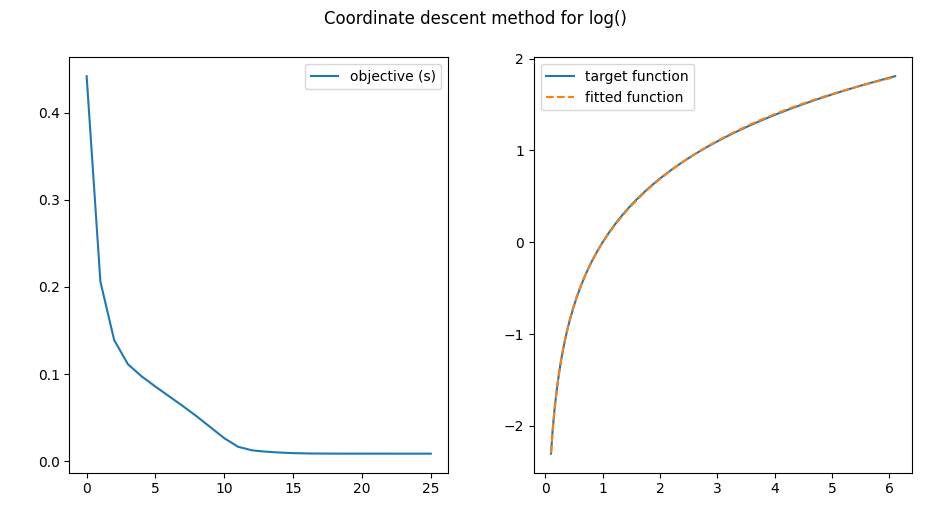
print("\nCoordinate descent method")
cdp = CoordinateDescentFitProblem()
cdp.create_problem()
cdp_steps, cdp_time, cdp_obj_vals = cdp.solve(1)
print("Coordinate descent took", cdp_steps, "iterations and", 
    "{0:0.3f}".format(cdp_time), "ms to solve the problem")
print("Attained objective value is", cdp.evaluate_objective())

fig, ax = plt.subplots(1, 2)
plt.suptitle("Coordinate descent method")
fig.tight_layout()
ax[0].plot(cdp_obj_vals, label = "objective (s) vs iteration number")
ax[0].legend()
ax[1].plot(cdp.t, cdp.y, label = "target function")
ax[1].plot(cdp.t, cdp.fitted_fun(), linestyle = "dashed", label = "fitted function")
ax[1].legend()
plt.show()

The plot showing up as result of running this script should look like the one below.

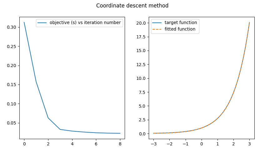
I call it a success. Visually, this is a pretty good fit ;-)

Imperative to the success is the fact that the attained objective values decrease with each iteration. They could not go up and it is a feature of coordinate descent algorithms. Indeed, the first step solves a feasibility problem that finds values of \(\vec{a}\) and \(\vec{b}\), such that the fit error is in the \([0, s_p]\) range, while the second LP is set to minimize \(s\), hence the resulting objective value \(s^*\) will be no greater than \(s_p\), which, as we already know from the first step, is attainable. Essentially, the first step finds \(\vec{b}\) that would satisfy the \(s_p\) and the second step, given the current value of \(\vec{b}\), attempts to decrease \(s\) (by changing \(\vec{a}\)). This is the reason why the iterative process converges.

Performance-wise, the result is also nothing to sneeze at:

1
2
3
Coordinate descent method
Coordinate descent took 10 iterations and 0.054 ms to solve the problem
Attained objective value is 0.022732236042735998

The performace is comparable to that of bisection. It so happens, coordinate descent completed in the same number of steps as did bisection, but took (roughly) twice as long to do the computation: after all, we are solving two optimization problems per step, not one. The running time is higher, but so is the accuracy. We have achieved a higher (though only marginaly so on account of the bisection implementation being very precise to begin with) accuracy without encounering any numerical issues!

In fact, this algorithm turned out to be numerically robust with relation to variation in initial values as well. Why not take advantage of this “bonus feature” and see how number of iterations depends on initial value of \(s\)?

1
2
3
4
5
6
7
8
9
10
11
12
13
14
15
16
17
18
19
cdp = CoordinateDescentFitProblem()
cdp.create_problem()

#optimal objective value is about 0.0227; setting s lower than that will produce an infeasible problem
siv = np.concatenate((np.linspace(0.03, 0.1, 10), np.linspace(0.1, 1, 10)))
sts = np.zeros(len(siv))
obs = np.zeros(len(siv))
for i in range(len(siv)):
    cdp_steps, _, _ = cdp.solve(siv[i])
    sts[i] = cdp_steps
    obs[i] = cdp.evaluate_objective()

print("Avarage optimal objective:", "{0:0.5f}".format(np.mean(obs)), 
    "with st. deviation", "{0:0.7f}".format(np.std(obs)))

plt.plot(siv, sts, label = "number of iterations vs initial value for s")
plt.title('Coordinate descent method')
plt.legend()
plt.show()

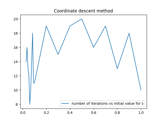
Surprisingly, the relationship is not a monotonically increasing one, rather, it exhitits a “dome-shaped” tendency. Getting to the bottom of this mystery might prove an engaging edeavour, but this is an exercise for some other time. In the end, it is reassuring to know that whatever (reasonable) initial value one chooses, the algorithm will not end up in an exception handler.

Finally, to be on a safe side, let us make sure our implementation works equally well with some other objective, say, \(log(x)\).

1
2
3
4
5
6
7
8
9
class CoordinateDescentFitProblemForLog(CoordinateDescentFitProblem):

	def define_domain_bounds(self):
		self.k = 201
		self.lb = 0.1
		self.ub = 6.1

	def function_to_fit(self, x):
		return np.log(x)

All in all, coordinate descent appears to be a decent alternative to bisection.

Flawed Variant of Iterative Partial Minimization

Each, bisection and coordinate descent, may be considered a particular case of the general technique I call iterative partial minimization (the term is of my own devising) that consists in minimizing over a subset of variables in an iterative manner, the difference between the two being that coordinate descent alternates between optimizing over multiple subsets of variables, whereas bisection minimizes over all variables but one and the value of remaining variable is determined by binary search. Both methods work equally well.

Why not, for the sake of completeness and to indulge one’s curiosity, try out an approach that does not or, at least, is not supposed to work? Take another look at the problem.

Recall from the previous discussion that the terms responsible for non-convexity are \(s \cdot b_1\) and \(s \cdot b_2\). Let us try and eliminate them.

“Wait a minute,” I can already hear a protest coming my way, “that did not get rid of non-convexity; the liable terms were just shifted down, to other constraints.” Well, we are not done yet. Iterative partial minimization solves the original problem almost “as is”, with the only difference that some of the variables are turned into parameters. We will take this idea one step further (or a step too far if you will), partitioning constraints also. In particular, the algorithm will alternate between solving two problems:

and

Anyone who wishes to see the implementation should look for the class FlawedPartialMinimizationFitProblem in my python script. Code-wise, it is not that much different from the previous two algorithms (so I will not give a function by function walk-through this time). There are few points of interest, however.

First of all, solution to the LP at the first step may violate the constraints of the original problem, because in the inequalities \(a_0 + a_1 \cdot t_i + a_2 \cdot t_i^2 - y_i \cdot z_i \le s + b_{1,s} \cdot t_i + b_{2,s} \cdot t_i^2\) and \(a_0 + a_1 \cdot t_i + a_2 \cdot t_i^2 - y_i \cdot z_i \ge -s - b_{1,s} \cdot t_i - b_{2,s} \cdot t_i^2\) the right-hand sides are checked against the expressions computed w.r.t constant parameters \(b_{1,s}, b_{2,s}\) (not the current values of \(b_1\), \(b_2\)); as a result, the attained objective value will underestimate that for the original problem. We will keep track of objective values for the modified and original problems and record by how much the constraints are violated.

Second of all, not one, but two initial values for the parameters are now required and there is no clear limit on how high or low they can be.

Finally, divided into non-intersecting partitions, the constraints from different groups tend to “pull” the solution back and fourth in opposite directions thus resulting in oscillations and, as a consequence, the iterative process never converges. In order to avoid an infinite loop, we impose a limit on the number of iterations and use it as an additional termination criterion.

As before, we are placing the original and fitted curves on a single plot to evaluate the quality of interpolation. In addition to that, the stats concerning attained objective values for the original and modified problems are depicted on a separate plot to illustrate a point presented in the earlier discussion.

Here are the plots:

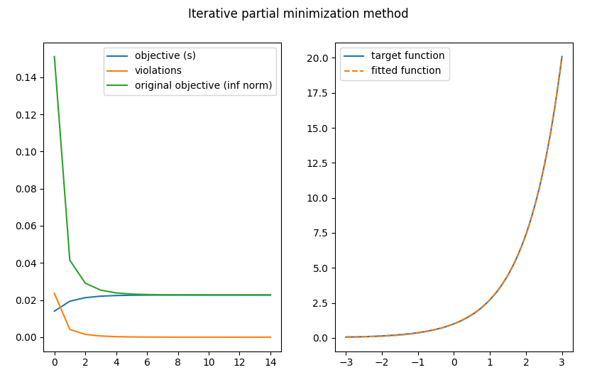
What do we observe? Visually, the fitted curve matches our target function well. With each iteration, the magnitude of violations decreases (going to zero) and the attained objective value for the LP at step 1, while initially underestimating it (as was predicted), converges to the optimal objective value for the original problem. We did not need that precautionary limit on the number of steps after all.

Now a few words on the subject of performance.

1
2
Iterative partial minimization took 16 iterations and 0.091 ms to solve the problem
Attained objective value is 0.022726816104874814

As compared to bisection and coordinate descent, this algorithm took more time and iterations to obtain the solution with the same, high, accuracy, but not by much. The number of iterations does increase if we choose “unlucky” initial values for \(b_{s,i}\), but, again, not drastically (within a factor of 4), as convincingly demonstrated by the heatmap below.

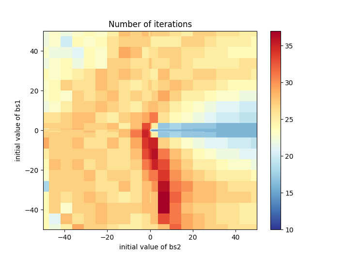
Here is the python script that constructs this heamap.

1
2
3
4
5
6
7
8
9
10
11
12
13
14
15
16
17
18
19
#Genearing the heat map llustrating dependency between number of iterations and initial values for the problem parameters
init_vals = np.concatenate((np.linspace(-50, -1, 10), np.linspace(-1, -0.1, 10), np.linspace(-0.1, -0.01, 10), 
np.linspace(0.01, 0.1, 10), np.linspace(0.1, 1, 10), np.linspace(1, 50, 10)))
stephm = np.zeros((len(init_vals), len(init_vals)))
for i in range(len(init_vals)):
    for j in range(len(init_vals)):
        st, _, _, _,_ = pmp.solve(init_vals[i], init_vals[j])
        stephm[i, j] = st

x, y = np.meshgrid(init_vals, init_vals)

fig, ax = plt.subplots()
cmsh = ax.pcolormesh(x, y, stephm, cmap = 'RdYlBu_r')
ax.set_title('Number of iterations')
ax.axis([x.min(), x.max(), y.min(), y.max()])
plt.ylabel('initial value of bs1')
plt.xlabel('initial value of bs2')
fig.colorbar(cmsh, ax = ax)
plt.show()

Notice that the \(b_{s,i}\)’s values range over non-linear space with the density of points inreasing near zero; by so doing I test how the algorithm behaves if parameters are initialized to small values. There is no natural boundary on the value \(s \cdot b_i\) can take, but given that \(s\) is expected to be close to zero, \([-50, 50]\) seems more than enough.

Hopefully, it has not escaped reader’s notice that, while generating the heatmap, we were able to solve multiple instances (with a variety of initial conditions) of the problem without rasing an exception. Not only is the method numerically stable with relation to an increasing target accuracy, but also, to variations in initialization values for the parameters.

Is this aglorithm great, or what?! But was not there an inherent flaw to it? How come it works? Well, it does not! Look at what happens if we apply the same method to the task of fitting another function – \(log(x)\), for example.

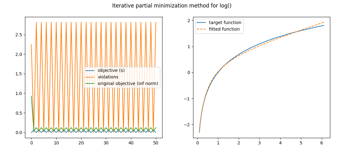
These are the oscillations I mentioned earlier. The iterative process does not converge! Ultimately, this is not a viable approach.

Conclusion

I bet, reading all this has put you to sleep. Wake up! The “oh no, not another school paper” is nearly over. Preparing the post, indeed, reminded me of the time I wrote school reports that most people would find boring, my only hope being that goofy bookish phraseology and colloquial expressions appearing here and there thoughout the text would make it feel sligtly less so.

Presented in this work are three methods of solving the minimax rational fit to the exponential, all unifiable under an unofficial umbrella term of iterative partial minization. Of these, only bisection and coordinate descent are viable. Bisection and coordinate descent are comparable in terms of performace, bisection taking less time to find the solution with the requested accuracy 0.001, but exhibiting numerical issues (that coordinate descent does not suffer from) where a higher acuracy is required. The third method seems to work at first glance, however its design has an inherent flaw to it. The method was presented to warn the reader about a potential pitfall.

– Ry Auscitte

References

1. Cvxpy: A Python-embedded modeling language for convex optimization problems.
2. ECOS: A lightweight conic solver for second-order cone programming.
3. Stephen Boyd, Convex Optimization, Stanford Online.
4. John W. Paisley, Machine Learning, Columbia University.
5. Stephen Boyd and Lieven Vandenberghe (2004), Convex optimization, Cambridge university press.
6. Stephen Boyd and Lieven Vandenberghe, Additional Exercises for Convex Optimization
7. Christopher M. Bishop (2006), Pattern Recognition and Machine Learning, Springer New York
8. Desmos: Graphing Calculator
9. Alexander Domahidi, Eric Chu and Stephen Boyd (2013), ECOS: An SOCP solver for embedded systems, 2013 European Control Conference (ECC), 2013, pp. 3071-3076
10. Finding solution to quasi-convex problem using CVXPY