Decision Trees: a Mysterious Case of Increasing Cross-Entropy Loss
Introduction
The other day I came across an old machine learning project of mine; in yearning for the times that would never come back was I spending lonely hours of that evening while looking through those dated Jupyter notebooks. A travel down the memory lane was interrupted, however, by a curios phenomenon seizing my attention and, having given the idea some consideration, I decided it merited an investigation of its own, which I am presenting in this post.
A key step in nearly every machine learning project is overfitting diagnostics with learning and validation curves being the tools developers find handy in accomplishing the task. About the former, one can read in Andrew Ng’s very accessible Machine Learning Yearning. However, it was the latter that I chose to employ.
NOTE: The remainder of this and the section that follows are intended as a review of the machine learning concepts used later in the post. Those of my readers whose memory is their loyal servant, may skip to the main section of the work.
Before going into detail, it seems constructive to briefly remind the reader what overfitting is. In general terms, supervised machine learning concerns itself with fitting some form of a (multivariable and, quite often, highly complicated) function \(f\) to a \(n\)-sized sample (\(\mathbb{X}\)) of datapoints from \((d+1)\)-dimensional space (\(D_1 \times \dots \times D_{d+1}\)): \(f(x_1^{(i)},\ldots,x_d^{(i)}) \approx x_{d+1}^{(i)}, i = 1,\ldots,n\), so that, should we encounter a new point \(z\) with unknown value in the \((d+1)^{th}\) dimension, we could “predict” the latter as \(f(z_1,\ldots,z_k)\). (The first \(d\) components are called “features” and the one predicted – “outcome”/”response variable”). The function being fitted varies depending on the model used: from a simple affine relation \(\beta_0 + \beta_1 \cdot x_1 + \ldots + \beta_d \cdot x_d\) of linear regression to \(sign(\beta_0 + \beta^T \cdot \phi(x_{1:d}))\) (where \(\phi()\) is infinite-dimensional) of RBF SVMs or a recursive multilayered structure composed of linear combinations passed to non-linear activation functions, which is at the heart of even the simplest neural networks, and everything in between.
Implementation of this reasonable-sounding idea, when faced with the harsh reality, present two major challenges: firstly, the sample of datapoints is of finite (albeit, maybe, very large) size and, therefore, it is difficult to tell which regularities are specific to the sample and which are characteristic of the entire population; and secondly, the real-world data may not quite adhere to the idealized relation specified by \(f\). As a result, the function is chosen such that it would pick up only the general tendencies in the data, a justification for which can be found in the statistical interpretation of machine learning models. Now there are random factors to explain the misfits. For example, linear regression assumes the vectors \(\{(x_1^{(i)}, \ldots, x_d^{(i)}, x_{d+1}^{(i)}) \mid i = 1,\ldots,n\}\) actually conform to the affine relation, but their last components, \(x_{d+1}^{(i)}\), are subject to random measurement errors. One’s task is to recover the hidden relation while ignoring the measurement noise. In this setting, choosing a function, complex enough so as to reflect the randomness, would be considered an “overfitting” since it will likely be off by a large amount when computed for some new datapoint that has not been “seen” by the fitting procedure. On the other hand, the function must be complex enough to represent the underlying structure of data well. Continuing our regression analysis example, when a linear relation is not a good fit, one might have to extend the vectors with powers of existing components: \((x_1, \ldots x_d, x_1^2, \ldots x_d^2, x_1^3, \ldots x_d^3, \ldots, x_1^p, \ldots x_d^p, x_{d+1})\), thereby transitioning into the realm of polynomial regression.
So how does one know when enough is enough? How is one to select a model of proper complexity? This is when validation curves come into play. To plot one, two things must be defined:
- A quantitative measure of model complexity (for polynomial regression, it would be the degree of polynomial \(p\)). Its values will run along the \(x\) axis.
- A performance metric. They come in two flavors: a measure for the goodness of fit (such as accuracy), that computes to higher values for better fits, and a loss function, that quantifies the fitting error, and, as such, decreases as the quality of fit goes up. Values of the performance metric is what ticks on the \(y\) axis will correspond to.
Then the data sample \(\mathbb{X}\) is divided into two disjoints subsets: a training and validation datasets. For a series of models of increasing complexity, we will fit the underlying function \(f\), parameterized by the current value of complexity measure, to the training dataset and then evaluate its performance on the training and validation datasets, thereby producing two curves encompassed by the common term “validation curves”. What one expects to see is continuous improvement in performance on the training dataset all the way up; as to the validation dataset, once the model starts detecting the regularities specific to the training data (and, therefore, not present in the validation dataset), the performance will drop, as will be indicated by the corresponding validation curve changing its course (i.e. starting to decrease if the metric characterizes goodness of fit, or increase if a loss function has been chosen). Once it happens, the model has become “too complex” (of course, validation curves may fluctuate slightly due to mismatch in optimization criteria; what is actually examined is the general trend).
This work investigates a peculiar behavior of validation curves constructed for a validation dataset and, hopefully, the few short paragraphs above gave a proper introduction to the subject matter.
The Dataset and Metrics
Every machine learning project needs a dataset. Let me present the one I used.
All Windows executable files - applications, dynamic-linked libraries, and drivers - adhere to the Window portable executable (PE) format. Header section of the executable file is usually filled in by the linker and differs from file to file depending on the specifics of the program. It contains such information as the target platform, linker version, table of imported functions, sizes of stack and heap, etc. Mauricio Jara requested a collection of malware executable modules from virusshare, then run a PE parsing utility against the malware collection and clean files, Windows system files and well-known applications, and made the resulting dataset freely available online. The dataset contains 19612 samples, each described by 79 features.
This dataset was designed for use in training machine learning models to predict whether a software sample is benign or malware based on the data stored in PE headers of its executable file, hence before us is a classification problem with a categorical outcome variable and two classes (categories, labels): Benign (0) and Malware (1), i.e. \(f: D_1 \times \dots \times D_d \rightarrow \{0, 1\}\). Which performance metrics are applicable in this case? (Classification) accuracy, a proportion of correctly classified datapoints, is, of course, a staple
\[acc(\mathbb{X}) = \frac{1}{n} \cdot \left| \{ i \mid f(x_1^{(i)},\ldots,x_d^{(i)}) = x_{d+1}^{(i)},\; i=1,\ldots,n\} \right|\]Another metric for classification problems is cross-entropy loss. It is used in a probabilistic setting, where \(f\) is defined slightly differently: \(f: D_1 \times \dots \times D_d \rightarrow [0, 1]^{c-1}\), with \(c\) being the number of classes and the codomain \([0, 1]^{c-1}\) – the vectors of predicted probabilities of \(x_{d+1}\) belonging to the classes \(0, 1, \ldots, c-2\). That is, instead of one, concrete, class, \(f\) predicts a probability spread over all classes, the interpretation being: given the features \(x_1,\ldots,x_d\), the probability that \(x_{d+1}\) belongs to the category \(k\) is \(f_{k+1}(x_1,\ldots,x_d)\). Naturally, one must define an order on the classes and set
\[P(x_{d+1} \in c - 1) = 1 - \sum_{i=0}^{c-2} P(x_{d+1} \in i)\]Then, the cross-entropy loss is computed as follows:
\[cel(\mathbb{X}) = \frac{1}{n}\sum_{i = 1}^{n}\left[ - \sum_{k = 0}^{c-1} \unicode{x1D7D9} \{x^{(i)}_{d+1} = k\} \cdot logf(x_1^{(i)}, \ldots, x_d^{(i)})\right]\]Cross-entropy loss is closely related to the notion of cross entropy. Given two discrete probability distributions over the same finite support with PMFs specified by the vectors \((p_1,\ldots,p_n)\) and \((q_1,\ldots,q_n)\) respectively, cross entropy is
\[H(p,q) = - p_i \cdot \sum_{i = 1}^{n} log q_i\](the units differ depending on the logarithm’s base; in machine learning, they use natural logarithms and cross-entropy is measured in nats). The concept comes from information theory, where it measures an average number of nats needed to represent a randomly chosen value by the encoding scheme constructed for probabilities \(\{q_i\}\) when its true distribution is determined by \(\{p_i\}\). Returning to the classification problem, the true distribution of \(x_{d+1}\) is
\[\begin{gather*} p_i = \begin{cases} 1 & \text{if } i = x_{d+1}\\ 0 & \text{otherwise} \end{cases} \end{gather*}\]and \(\{q_i\}\) are computed by \(f\). Thus, the farther apart \(\{p_i\}\) and \(\{q_i\}\) are, the larger the cross entropy is or, from a different angle, the poorer the fit, the larger the cross-entropy loss is. What is more, in this setting, cross entropy computes the same value as Kullback–Leibler divergence, a widely-used measure of distance between two distributions.
For binary classification, it is natural to identify the “true” class or, in other words, a property the datapoint is “tested for”. Is this module a malware? Is this patient likely to have a heart attack? This class is put first in the order on classes and, thus, \(f: D_1 \times \dots \times D_d \rightarrow [0, 1]\) computes the probability of “testing positive”. Let us rewrite the cross-entropy loss for the case of two classes:
\[cel(\mathbb{X}) = \frac{1}{n}\sum_{i = 1}^{n}\left[- x^{(i)}_{d+1} \cdot log f(x^{(i)}_1, \ldots, x^{(i)}_d) - (1 - x^{(i)}_{d+1}) \cdot log(1 - f(x^{(i)}_1, \ldots, x^{(i)}_d))\right]\]Speaking of binary classification, there is a special model designed specifically for solving this kind of problems; it goes by the name of logistic regression. Behind the way this model constructs \(f\) is a statistical interpretation of \(\mathbb{X}\). Logistic regression treats \(x_{d+1}\) as a random Bernoulli variable, i.e.
\[x^{(i)}_{d+1} | x^{(i)}_{1},\ldots,x^{(i)}_{d} \stackrel{ind}{\sim} Ber\left(p = \frac{1}{1 + exp(-\beta_0 - \beta_1 \cdot x_1^{(i)} - \ldots - \beta_d \cdot x_d^{(i)})}\right)\]that being the case, the probability of \(x_{d+1} = 1\) is calculated as follows
\[P(x_{d+1} = 1 \mid p) = p^{x_{d+1}} \cdot (1 - p)^{1 - x_{d+1}}\]Taking into account that \(x^{(i)}_{d+1}\) are assumed to have been sampled independently, one can compute the likelihood of the entire dataset \(\mathbb{X}\) as
\[L(p) = P(\mathbb{X}_{[:,d+1]} = 1 | \mathbb{X}_{[:,1:d]}) = \prod_{i=1}^{n} p^{x^{(i)}_{d+1}} \cdot (1 - p)^{1 - x^{(i)}_{d+1}}\]and then, find a maximum likelihood estimator for \(p\) using the well-known trick of eliminating products by taking \(log\) (a monotonically increasing function).
\[logL(p) = l(p) = \sum_{i=1}^{n} x^{(i)}_{d+1} \cdot logp + (1 - x^{(i)}_{d+1}) \cdot log(1 - p)\]Why not minimize \(-l(p)\) instead of maximizing \(l(p)\)? Then one can talk about a loss function, which, in the framework of logistic regression, is referred to as “logistic loss” or, simply, “log-loss”.
To sum up, logistic regression fits the function \(f(x_1,\ldots,x_d) = p = \frac{1}{1 + exp(-\beta_0 - \beta_1 \cdot x_1 - \ldots - \beta_d \cdot x_d)}\) to the sample \(\mathbb{X}\) using the log-loss loss function:
\[ll(\mathbb{X}) = -\sum_{i=1}^{n} x^{(i)}_{d+1} \cdot logf(x^{(i)}_1,\ldots,x^{(i)}_d) - (1 - x^{(i)}_{d+1}) \cdot log(1 - f(x^{(i)}_1,\ldots,x^{(i)}_d))\]Multiplying by a constant will not change the argmin, therefore the loss function can be rewritten as:
\[ll(\mathbb{X}) = \frac{1}{n}\left[\sum_{i=1}^{n} - x^{(i)}_{d+1} \cdot logf(x^{(i)}_1,\ldots,x^{(i)}_d) - (1 - x^{(i)}_{d+1}) \cdot log(1 - f(x^{(i)}_1,\ldots,x^{(i)}_d))\right]\]It should not have escaped the reader’s notice, that formulae for log-loss and binary cross-entropy look identical. Indeed, these are the two measures, different in nature, but amounting to the same computation steps. Considering that our classification problem is binary, the terms “log-loss” and “cross-entropy loss” will be used interchangeably. For more information on the subject of cross-entropy and log-loss metrics (as well as the relationship between them), see online publications by Jason Brownlee (here) and Lei Mao (here and here).
Having established which performance metrics suit the problem, now comes the time to settle the question of measure for model complexity. To do that, one must first decide on the model. I have already given my choice away by stating it in the title – Decision Tree – and it might have come as a surprise to many. Admittedly, decision trees have fallen out of fashion with the emergence of new, more sophisticated, classifiers, but this model is simple, fast, works well with small datasets, and requires no preprocessing. It is definitely still worth studying, at the very least, as a building block for the high-performing ensemble classifiers such as random forests.
Decision Trees specify the function (\(f\)) being fitted in the form of a tree structure similar to the one on the figure below (in special cases, \(f\) can be defined in a closed form: for example, when there are two classes only and probabilities are not needed, that is, \(f\) returns a zero-based class index, it is a boolean function).
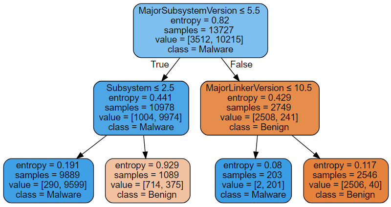
Computing \(f\) is a simple matter. Suppose, one is given a datapoint with MajorSubsystemVersion = 6 and MajorLinkerVersion = 9, then following the conditions printed at the top on the nodes (see the figure), the datapoint will end up in the third leaf from the left. Assigned to this leaf are 2 benign and 201 malware instances (see the value field), therefore the datapoint is predicted to be malware with the probability \(201/(2 + 201)\). As is, if we always choose the class with the highest probability of the two, the model will mistaken in 290 + 375 + 2 + 40 cases out of 13727. It is not the perfect fit! By splitting the leaves further (on some conditions, other than MajorSubsystemVersion <= 5.5, Subsystem <= 2.5, etc.), one can raise the number of points belonging to the prevalent class until, possibly, instances of one class only remain. Obviously, growing the tree improves the quality of fit. On the whole, limit on the tree depth is a good quantitative measure of the Decision Tree model complexity and this is what we are going to use.
On this note, I am completing the introductory section of the post. Of course, the reader steeped in machine learning must have known all this already. Nevertheless, I hope, this section served as an effective review of the key concepts, at the same time, putting everyone, including machine learning newbies, on equal footing.
The Phenomenon, at your Service
The theory review done and dusted, we can proceed to the more exciting investigative part of the work, and the reader is invited to join in the endeavor. As per tradition, I am omitting the plotting-related code as non-essential to understanding the experiments, but it can still be found in the notebook, available on github and kaggle.
The “subject” of our “investigation” will be introduced in the course of a simple experiment; scikit-learn (sklearn for short) is the machine learning framework of choice for this experiment. We begin by loading the dataset and splitting it into training and validation subsets. (The same deterministic random state will be passed to all the functions where it is applicable throughout the notebook to ensure reproducibility of the experimental results.)
1
2
3
4
5
6
7
8
9
10
11
12
13
import pandas as pd
import numpy as np

data = pd.read_csv("dataset_malwares.csv")

from sklearn.model_selection import train_test_split

rs = 42
X_train, X_val, y_train, y_val = train_test_split(
                                     data.drop(["Name", "Malware", "CheckSum"],
                                               axis = 1),
                                     data["Malware"], test_size = 0.3,
                                     random_state = rs)
The validation subset is then used to construct validation curves for a progressing (i.e. gradually changing in one direction) value of some model parameter. This work studies decision trees with an increasing limit on the maximum tree depth, but we are allowing for an arbitrary model and (a set of) parameter(s).
Further pursuing the versatility objective, arbitrary statistics for a sample of predicted and actual labels, of which classification performance metrics are a special case, are computed (multiple at a time, for the added benefit of performance). All of this is accomplished with the help of python’s function objects: create_classifier() accepts an integer in some way identifying the value(s) of model parameter(s) and is expected to return a sklearn’s estimator; list_initializers is a list of function objects computing the statistics. collect_statistics() returns a tuple of lists, each holding a sequence of values for a statistic (one sequence element for every value of the model parameter). The way collect_statistics() works will become clear once you see it used in practice.
stat_range is meant to identify a sequence of parameter values for the chosen model. In reality, it is only a sequence of integers (that starts with 0) and it is create_classifier’s responsibility to translate an element of stat_range to the value of the model parameter in order to create a properly parameterized :-) model.
1
2
3
4
5
6
7
8
9
10
11
12
13
14
15
16
17
18
19
20
21
stat_range = range(30)

def collect_statistics(create_classifier, list_initializers,
                       Xtrain = X_train, ytrain = y_train,
                       Xval = X_val, yval = y_val):

    stats = [ [] for l in range(len(list_initializers)) ]

    for i in stat_range:
        model = create_classifier(i)
        model.fit(Xtrain, ytrain)

        y = model.predict(Xval)
        p = model.predict_proba(Xval)
        p0 = p[yval == 0, 0]
        p1 = p[yval == 1, 1]

    for l in zip(stats, list_initializers):
        l[0].append(l[1](y, p, p0, p1))

    return tuple(stats)
Next we define a function object that creates an instance of the decision tree model with a limit on its tree depth (starting with a depth of 2) given by the (only) argument x.
1
2
3
4
cart_depth_lim = lambda x: DecisionTreeClassifier(criterion = "entropy",
                                                  max_depth = x + 2,
                                                  random_state = rs)
cart_depth_lim_depths = lambda x: [ i + 2 for i in x ]
With all the preliminary work out of the way, let us finally plot a validation curve for an increasing limit on the tree depth with log-loss as a performance metric (alongside the same but with the classification performance evaluated by computing its accuracy).
1
2
3
atrs, lsrs = collect_statistics(cart_depth_lim,
                 [ lambda y, p, p0, p1: accuracy_score(y_val, y),
                   lambda y, p, p0, p1: log_loss(y_val, p) ] )
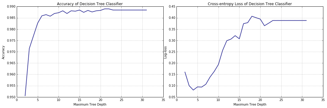
The accuracy increases with the model improving in its capacity to fit the data (as it should). Surprisingly, beginning from a depth limit of 5, cross entropy, that hitherto has been predictably decreasing, suddenly turns 180 degrees and starts growing. What is happening? Well, validation curve can change its curse “for the worse” as a result of overfitting; however, it does not seem to be the case here: firstly, a five-level-deep decision tree is not complex enough to overfit the training data we have and, secondly, the accuracy-based validation curve does not display a matching tendency.
Hypothesis I: a Trade-off Between Precision and Recall
Our experience tells us: anomalies in the behavior of classification performance metrics can sometimes be explained by an interplay between precision and recall, which are changing along with the model complexity.
Obviously, drops in classification performance come as a result of classification errors. With only two categories at its disposal, there are not many ways the classifier can be wrong: either it misclassifies a malicious software as benign (let us call it a “false negative”) or takes a perfectly innocent benign module for a malware (which is dabbled a “false positive”, by analogy).
Following the notation introduced in the previous sections, we can define the number of false positives and false negatives (as well as their “errorless” counterparts) as statistics for the dataset \(\mathbb{X}\).
\[fp(\mathbb{X}) = \left| \{ i \mid f(x_1^{(i)},\ldots,x_d^{(i)}) \ge 0.5 \;\&\; x_{d+1}^{(i)} = 0,\; i=1,\ldots,n\} \right| \quad \text{(false positives)}\] \[fn(\mathbb{X}) = \left| \{ i \mid f(x_1^{(i)},\ldots,x_d^{(i)}) < 0.5 \;\&\; x_{d+1}^{(i)} = 1,\; i=1,\ldots,n\} \right| \quad \text{(false negatives)}\] \[tp(\mathbb{X}) = \left| \{ i \mid f(x_1^{(i)},\ldots,x_d^{(i)}) \ge 0.5 \;\&\; x_{d+1}^{(i)} = 1,\; i=1,\ldots,n\} \right| \quad \text{(true positives)}\] \[tn(\mathbb{X}) = \left| \{ i \mid f(x_1^{(i)},\ldots,x_d^{(i)}) < 0.5 \;\&\; x_{d+1}^{(i)} = 0,\; i=1,\ldots,n\} \right| \quad \text{(true negatives)}\]A likely consequence of parameter tweaking is that the classifier shifts from one type of error to another; precision and recall are used to keep track of these shifts (among other things). Precision calculates a percentage of veritably malicious modules out of all classified as such, whereas recall is a proportion of malicious modules labeled “Malware” to all the malware in the dataset.
\[prec(\mathbb{X}) = \frac{tp(\mathbb{X})}{tp(\mathbb{X}) + fp(\mathbb{X})} \quad \text{(precision)}\] \[rec(\mathbb{X}) = \frac{tp(\mathbb{X})}{tp(\mathbb{X}) + fn(\mathbb{X})} \quad \text{(recall)}\]Let us plot the validation curves with precision and recall as performance metrics.
1
2
3
recs, precs = collect_statistics(cart_depth_lim,
                  [ lambda y, p, p0, p1: recall_score(y_val, y),
                    lambda y, p, p0, p1: precision_score(y_val, y) ] )
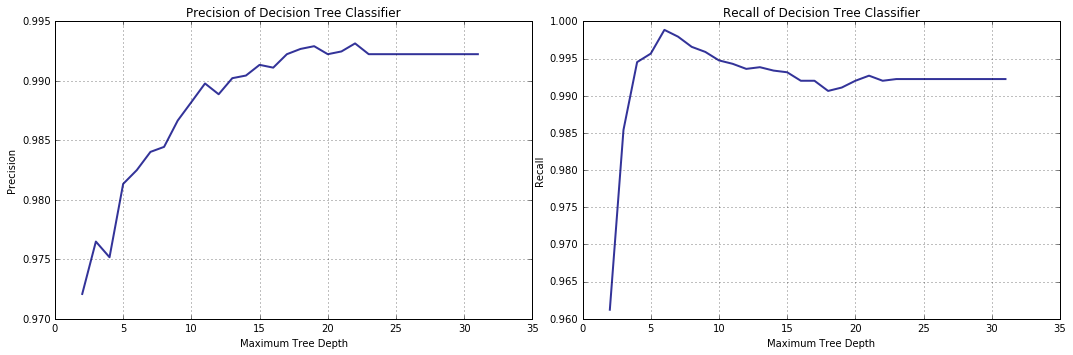
Indeed, precision and recall exhibit somewhat opposing behavior. What is more, recall starts decreasing pretty early on (thereby making the more accurate models worse in some sense) and, where malware detection is concerned, recall is of utmost importance, while false negatives are arguably more of a concern than false positives are, therefore the issue is worth our attention.
A cursory examination of the plots shows that recall is close to one at the tree depth just above 5, but we would do well to identify the (most likely) exact value of the parameter. For this purpose a 5-fold cross-validation procedure with the scoring metric set to “recall” will be used.
1
2
3
4
5
6
7
8
9
10
11
12
13
14
15
16
from sklearn.model_selection import GridSearchCV

parameters = { "max_depth" : cart_depth_lim_depths(stat_range) }
clf = GridSearchCV(DecisionTreeClassifier(criterion = "entropy", random_state = rs),
                   parameters, cv = 5, scoring = 'recall')
clf.fit(X_train, y_train)
best_max_depth = clf.best_params_['max_depth']
print("Best value of max_depth:", best_max_depth)

model_best_recall = DecisionTreeClassifier(criterion = "entropy", random_state = rs,
                                           max_depth = best_max_depth)
model_best_recall.fit(X_train, y_train)
yp = model_best_recall.predict(X_val)
print("Recall:", recall_score(y_val, yp))
print("Precision:", precision_score(y_val, yp))
print("Accuracy:", accuracy_score(y_val, yp))
Here is the output:
1
2
3
4
Best value of max_depth: 6
Recall: 0.9988594890510949
Precision: 0.982499439084586
Accuracy: 0.9858939496940856
The benefit of using a cross-valadation technique is that it eliminates (at least to some extent) randomness by averaging over multiple splits thereby uncovering true trends. Even so, the depth thus determined is relatively small. The resulting model will likely be biassed; heavily constrained or simplified models lack the capacity to pick up on all but trivial regularities in data. In the worst case scenario, such model simply predicts the prevalent class (complitely ignoring the features).
In this case the situation is not that bad; however, high recall with comparatively low values of both, precision and accuracy, suggests that predictions contain very few false negatives and signifiantly more false positives. One possible explanation is that the labels are unevenly distributed, i.e. skewed towards the Malware class. As a result, in many cases, the weak model exhibits a tendency to choose the majority class.
False positive and false negative predictions are easy to count.
1
2
3
4
from sklearn.metrics import confusion_matrix
tn, fp, fn, tp = confusion_matrix(y_val, model_best_recall.predict(X_val)).ravel()
print("Number of false positives:", fp)
print("Number of false negatives:", fn)
1
2
Number of false positives: 78
Number of false negatives: 5
The counts of false predictions seems to confirm our assumption. Let us now check if it was, in fact, correct.
1
2
3
4
5
print("Proportions of benign (negative) and malware (positive) binaries:",
      np.bincount(data["Malware"])/data.shape[0])
print("Null error rate:", np.bincount(data["Malware"])[0] / data.shape[0])
print("Error rate of the decision tree classifier:",
      1.0 - atrs[cart_depth_lim_depths(stat_range).index(best_max_depth)])
1
2
3
Proportions of benign (negative) and malware (positive) binaries: [0.25557085 0.74442915]
Null error rate: 0.2555708530926521
Error rate of the decision tree classifier: 0.014106050305914386
It was! There are significantly more Malware points (as compared to that belonging to the Benign class) in the dataset. Though the decision tree is still much more powerful than the primitive classifier always predicting the majority class (its error rate is called “null error rate”) as evident by the difference in the error rates.
How does this skew in label distribution affect structure of the decision tree?
1
2
3
4
5
6
7
8
9
10
11
12
13
14
15
16
17
18
19
20
21
22
23
24
25
26
27
28
29
30
31
32
33
34
35
36
37
38
39
40
41
42
43
44
45
46
47
48
import statistics as stat

def is_leaf(model, idx):
    return model.tree_.children_left[idx] < 0 and model.tree_.children_right[idx] < 0

def tree_stats(model):
    #leaves where the tree places each datapoint
    leaf_ids = model.apply(X_train)

    #predicted classes indexed by leaf ids (from class predictions for each leaf)
    leaf_preds = [ is_leaf(model, i) and
                   model.tree_.value[i][0][0] < model.tree_.value[i][0][1]
                   for i in range(len(model.tree_.value)) ]

    leaves_cnt = sum([ is_leaf(model, i) for i in range(len(model.tree_.value)) ])
    pls_cnt = sum(leaf_preds) #positive (benign) leaves
    nls_cnt = leaves_cnt - pls_cnt #negative (malware) leaves

    #total number of datapoints assigned to all negative leaves
    nls = sum([ e[1] for e in enumerate(model.tree_.n_node_samples)
                     if is_leaf(model, e[0]) and not leaf_preds[e[0]] ])
    #total number of datapoints assigned to all positive leaves
    pls = sum([ e[1] for e in enumerate(model.tree_.n_node_samples)
                     if is_leaf(model, e[0]) and leaf_preds[e[0]] ])

    elements, counts = np.unique(leaf_ids[y_train == 0], return_counts = True)
    tn = dict(zip(elements, counts)) #true negative
    elements, counts = np.unique(leaf_ids[y_train == 1], return_counts = True)
    tp = dict(zip(elements, counts)) #true positive

    #average number of misclassified datapoints per negative leave
    fn = stat.mean([ float(tp.get(i, 0)) for i in range(len(leaf_preds))
                                         if not leaf_preds[i] ])
    #average number of misclassified datapoints per positive leave
    fp = stat.mean([ float(tn.get(i, 0)) for i in range(len(leaf_preds))
                                         if leaf_preds[i] ])

    return (nls_cnt / leaves_cnt, nls/nls_cnt, fp),
           (pls_cnt / leaves_cnt, pls/pls_cnt, fn)

def print_tree_stats(model):
    (nsp, spnl, epnl), (psp, sppl, eppl) = tree_stats(model)
    print("            proportion   sample per    misclassified")
    print("            of leaves    leaf          samples per leaf")
    print("Benign SW: %10.5f" %nsp,"  %10.5f"%spnl, "  %10.5f"%epnl, " (false positive)")
    print("Malware  : %10.5f" %psp,"  %10.5f"%sppl, "  %10.5f"%eppl, " (false negative)")

print_tree_stats(model_best_recall)
1
2
3
4
            proportion   sample per    misclassified
            of leaves    leaf          samples per leaf
Benign SW:    0.44118    223.46667      8.63158  (false positive)
Malware  :    0.55882    546.05263      0.08333  (false negative)
In the decision tree, there are more leaves assigned “Malware” class (than “Benign”); per “Malware” leaf, there are more datapoints in the leaf, but fewer of them are classified incorrectly as compared to the “Benign” leaves, hence the model overall exhibits the tendency to prefer the “Malware” class in its predictions.
Tree Construction and Balanced Trees
Perhaps, it will be instructive to see how the tree is constructed and, in particular, how nodes are split using the first (root) node as an example. It may help better understand the role the distribution of labels plays.
1
2
3
4
5
6
7
8
9
10
11
12
13
from sklearn.tree import export_graphviz
import graphviz

dot_data = export_graphviz(model_best_recall,
                           max_depth = 1,
                           out_file = None,
                           feature_names = list(X_train.columns.values),
                           class_names=["Benign", "Malware"],
                           filled = True, rounded = True,
                           special_characters = True)

graph = graphviz.Source(dot_data)
graph
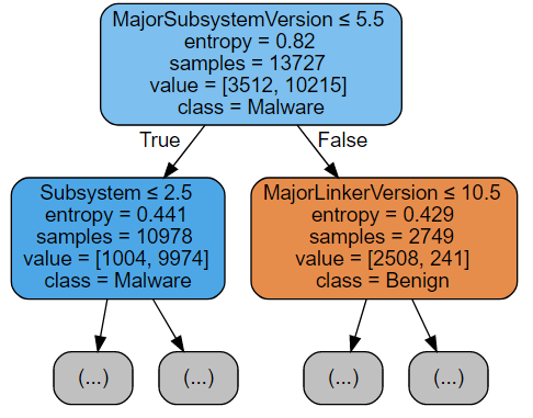
Examining the figure above, notice that at each non-leaf node the dataset split into two disjoints subsets in accordance with some condition (printed at the top of the rectangle depicting the node). The split criterion (the feature which to split on) as well as the threshold value are chosen such that the information gain, i.e. difference between the entropy of the parent node and a weighted (by the proportion of points of the assigned class in the subnode) sum of the entropies of its two children is maximized.
The entropy of a tree node is computed based on the frequentist estimate of the probabilities (p0 and p1) that a random point in this node is either malware (p1) or benign software (p0), or, simply put, on the frequencies of datapoints of each class. The chunk of code below performs the computation.
1
2
3
4
5
6
7
8
9
10
11
12
13
14
15
16
17
18
19
20
21
22
23
24
25
26
27
28
29
30
def log(x):
    return np.log2(x) if x != 0.0 else 0.0

def compute_entropy_unweighted(y):
    n0, n1 = np.sum(y == 0), np.sum(y == 1)
    p0, p1 = n0 / (n0 + n1), n1 / (n0 + n1)
    return (n0, n1, -p0 * log(p0) - p1 * log(p1))

def compute_gain(feature, threshold, compute_entropy, *args):

    print("Split condition for the node: ", X_train.columns[feature],
          "<=", threshold)

    divider = X_train.iloc[:, feature]
    y_left = y_train[divider <= threshold]
    y_right = y_train[divider > threshold]

    n0, n1, h = compute_entropy(y_train, *args)
    print("Source node: value = [", n0, ",", n1, "]; entropy = ", h)
    nl0, nl1, hl = compute_entropy(y_left, *args)
    print("Left node: value = [", nl0, ",", nl1, "]; entropy = ", hl)
    nr0, nr1, hr = compute_entropy(y_right, *args)
    print("Righ node: value = [", nr0, ",", nr1, "]; entropy = ", hr)

    return h - ((y_left.shape[0]/y_train.shape[0]) * hl +
                (y_right.shape[0]/y_train.shape[0]) * hr)

print("Gain = ", compute_gain(model_best_recall.tree_.feature[0],
                              model_best_recall.tree_.threshold[0],
                              compute_entropy_unweighted))
Below is the output one will get by running this code. Observe that the resulting entropy values match those displayed on the tree diagram.
1
2
3
4
5
Split condition for the node:  MajorSubsystemVersion <= 5.5
Source node: value = [ 3512 , 10215 ]; entropy =  0.8204132286187702
Left node: value = [ 1004 , 9974 ]; entropy =  0.4413099763029943
Righ node: value = [ 2508 , 241 ]; entropy =  0.42863845048023785
Gain =  0.38164088067497737
The same computation steps can be expressed in mathematical notation:
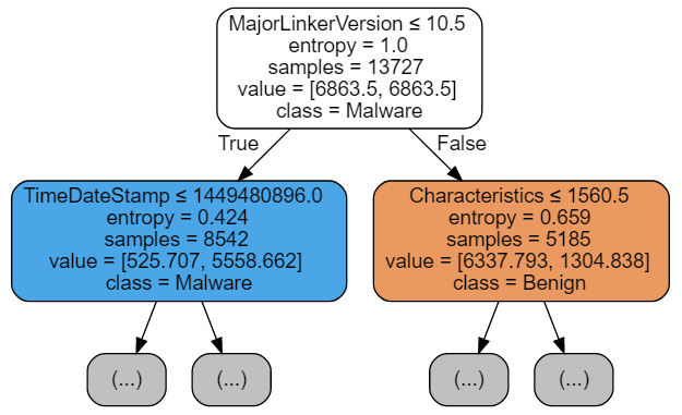
\[p1(\mathbb{X}) = \frac{\left| \{ i \mid x_{d+1}^{(i)} = 1,\; i=1,\ldots,\mid\mathbb{X}\mid\} \right|}{\mid\mathbb{X}\mid}\] \[H(\mathbb{X}) = - p1(\mathbb{X}) \cdot log(p1(\mathbb{X})) - (1 - p1(\mathbb{X})) \cdot log(1 - p1(\mathbb{X}))\] \[left(\mathbb{X}, sc, f) = \{\vec{x} \mid sc(x_f), \vec{x} \in \mathbb{X} \}\] \[right(\mathbb{X}, sc, f) = \{\vec{x} \mid \overline{sc(x_f)}, \vec{x} \in \mathbb{X} \}\] \[\begin{align*} gain(\mathbb{X}, sc, f) \;= \;&H(\mathbb{X}) - \frac{\mid left(\mathbb{X}, sc, f)\mid}{\mid\mathbb{X}\mid} \cdot H(left(\mathbb{X}, sc, f))\\ &- \frac{\mid right(\mathbb{X}, sc, f)\mid}{\mid\mathbb{X}\mid} \cdot H(right(\mathbb{X}, sc, f)) \end{align*}\]Designed specifically for datasets with uneven distribution of labels is balanced decision tree that is created by passing the class_weight argument set to “balanced” to the DecisionTreeClassifier’s constructor.
Let us take a look at the generated tree.
1
2
3
4
5
6
7
8
9
10
11
12
13
14
model_best_recall_bal = DecisionTreeClassifier(criterion = "entropy",
                                               random_state = rs,
                                               max_depth = best_max_depth,
                                               class_weight = "balanced")
model_best_recall_bal.fit(X_train, y_train)
dot_data = export_graphviz(model_best_recall_bal, max_depth = 1,
                           out_file = None,
                           feature_names = list(X_train.columns.values),
                           class_names=["Benign", "Malware"],
                           filled = True, rounded = True,
                           special_characters = True)

graph = graphviz.Source(dot_data)
graph
NOTE:
Let us ignore for now the fact that the TimeDateStamp feature found its way to the top tier, and that Characteristic, being an OR bitfield, should be treated differently. The topic of feature engineering, important as it is, lies beyond the scope of our discussion.
Notice that the number of datapoints assigned to the second-level nodes changed from (10978, 2749) to (8542, 5185) producing a more even split, which is accomplished by changing the way entropies are calculated. Below is a simplified version (the actual implementation is slightly more complicated) of the function that computes entropy. Therein, the frequencies used as estimates for the probabilities of a datapoint having Malware/Benign label are adjusted by class weights, each reverse proportional to the number of datapoints in the class. Though technically not completely correct, I like to think of it as datapoint counts for each class being adjusted to compensate for the uneven distribution of labels overall. To put it succintly, frequencies are corrected for the label imbalance.
1
2
3
4
5
6
7
8
9
10
11
weights = X_train.shape[0] / (2 * np.bincount(y_train))
print("Class Weights", weights)

def compute_entropy_balanced(y, w):
    n0, n1 = np.sum(y == 0) * w[0], np.sum(y == 1) * w[1]
    p0, p1 = n0 / (n0 + n1), n1 / (n0 + n1)
    return (n0, n1, -p0 * log(p0) - p1 * log(p1))

print("Gain = ", compute_gain(model_best_recall_bal.tree_.feature[0],
                              model_best_recall_bal.tree_.threshold[0],
                              compute_entropy_balanced, weights))
1
2
3
4
5
6
Class Weights [1.95429954 0.67190406]
Split condition for the node:  MajorLinkerVersion <= 10.5
Source node: value = [ 6863.5 , 6863.5 ]; entropy =  1.0
Left node: value = [ 525.7065774487471 , 5558.662310327949 ]; entropy =  0.4243475047893768
Righ node: value = [ 6337.793422551253 , 1304.8376896720508 ]; entropy =  0.6593753536591934
Gain =  0.48687713304918967
Mathematically, the only thing that changes is the way the probabilities are calculated:
\[w_0 = \frac{\mid\mathbb{X}\mid}{2 \cdot \mid\{ i \mid x_{d+1}^{(i)} = 0,\; i=1,\ldots,\mid\mathbb{X}\mid\}\mid}\] \[w_1 = \frac{\mid\mathbb{X}\mid}{2 \cdot \mid\{ i \mid x_{d+1}^{(i)} = 1,\; i=1,\ldots,\mid\mathbb{X}\mid\}\mid}\] \[p1(\mathbb{X}) = \frac{w_1 \cdot \left| \{ i \mid x_{d+1}^{(i)} = 1,\; i=1,\ldots,\mid\mathbb{X}\mid\} \right|}{\mid\mathbb{X}\mid}\]INFO:
By the way, notice that the balanced and regular trees are split on different feautures at the root node: MajorLinkerVersion and MajorSubsystemVersion respectively. For the most curious of my readers, plotted below are the information gain for both of them, computed in the setting of regular and belanced trees. It is easy to see that information gain for the split on MajorSubsystemVersion decreased, whereas the same for MajorLinkerVersion increased (at their respective maxima), which prompted the criterion change.
def compute_info_gain_range(ft):
   thr_seq = np.unique(X_train.iloc[:, ft])[:-1]
   gns, gnws = [], []
   gns = [ compute_gain(ft, t, compute_entropy_unweighted) for t in thr_seq ]
   gnws = [ compute_gain(ft, t, compute_entropy_balanced, weights) for t in thr_seq ]
   return thr_seq, gns, gnws`

fsq, gns, gnws = compute_info_gain_range(model_best_recall.tree_.feature[0])
fsq_b, gns_b, gnws_b = compute_info_gain_range(model_best_recall_bal.tree_.feature[0])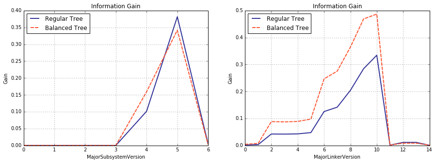
Let us run the print_tree_stats() once more, but this time for the balanced tree, and see what has changed.
1
2
3
4
            proportion   sample per    misclassified
            of leaves    leaf          samples per leaf
Benign SW:    0.47500    183.26316      4.61905  (false positive)
Malware  :    0.52500    487.85714      1.15517  (false negative)
There are still more leaves assigned a “positive” class in the tree; as before, Malware-labeled leaves contain more datapoint per leaf (after all, the data itself did not change – all the Malware had to go somewhere). What the new way of computing the entropy did is improving the balance between false positives and false negatives by redistributing the “positive” and “negative” datapoints among the nodes.
Now we shall see the effect the balancing had on precision and recall.
1
2
3
4
5
6
7
8
cart_depth_lim_bal = lambda i: DecisionTreeClassifier(criterion = "entropy",
                                                      class_weight = "balanced",
                                                      max_depth = i + 2,
                                                      random_state = rs)

recs_b, precs_b = collect_statistics(cart_depth_lim_bal,
                      [ lambda y, p, p0, p1: recall_score(y_val, y),
                        lambda y, p, p0, p1: precision_score(y_val, y) ] )
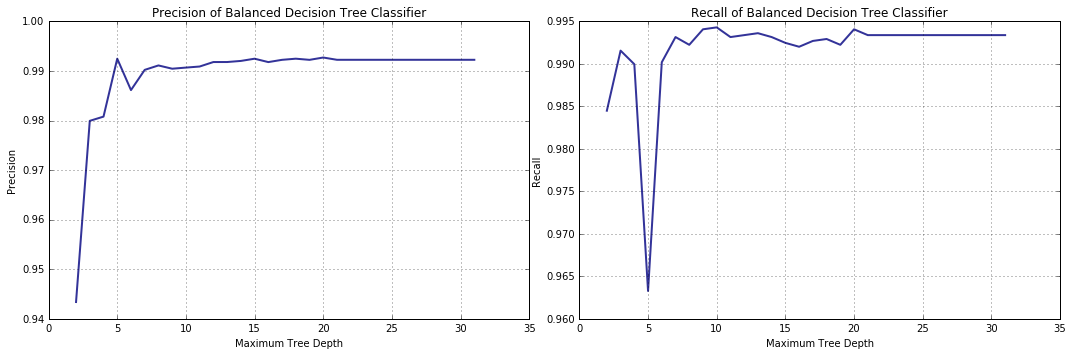
The recall score no longer displays a pronounced decrease trend as the limit on the tree depth grows.
NOTE:
As a side note, for the datasets with unbalanced labels, it is recommended to use balanced_accuracy() instead of accuracy(), provided all the classes are treated on equal footing. Validation curves for both are plotted below.
from sklearn.metrics import balanced_accuracy_score

#comma after batrs "unpacks" the tuple returned by collect_statistics()
batrs, = collect_statistics(cart_depth_lim,
	     [ lambda y, p, p0, p1: balanced_accuracy_score(y_val, y) ] )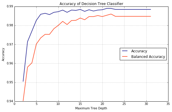
Sanity Check
I have some news for you – as luck would have it, good and bad. The good news is that we have found a solution for the falling recall problem. The bad news is that it is not the problem we were trying to solve. The recall’s decrease trend could not be the reason why cross entropy degrades due to magnitude of decrease in recall’s value not being high enough to overpower the raising precision. In particular, the log-loss formula is symmetric relative to the probabilities of each class, therefore it should be affected by both types of misclassification errors, false positives and false negatives, in equal measure. Another example of symmetry is F1 score and symmetric it is relative to the precision and recall values.
\[f1(\mathbb{X}) = 2 \cdot \frac{prec(\mathbb{X}) \cdot rec(\mathbb{X})}{prec(\mathbb{X}) + rec(\mathbb{X})}\]We will plot two validation curves: one, F1 score-based, for the regular decision tree, and another – the familiar log-loss, but for the balanced tree, and you will see that the recall trend, weak as it is, has no definitive effect on either.
1
2
3
4
5
6
7
8
9
10
f1s, = collect_statistics(cart_depth_lim,
                          [ lambda y, p, p0, p1: f1_score(y_val, y) ] )

cart_depth_lim_bal = lambda i: DecisionTreeClassifier(criterion = "entropy",
                                                      class_weight = "balanced",
                                                      max_depth = i + 2,
                                                      random_state = rs)

atrs_b, = collect_statistics(cart_depth_lim_bal,
                             [ lambda y, p, p0, p1: log_loss(y_val, p) ] )
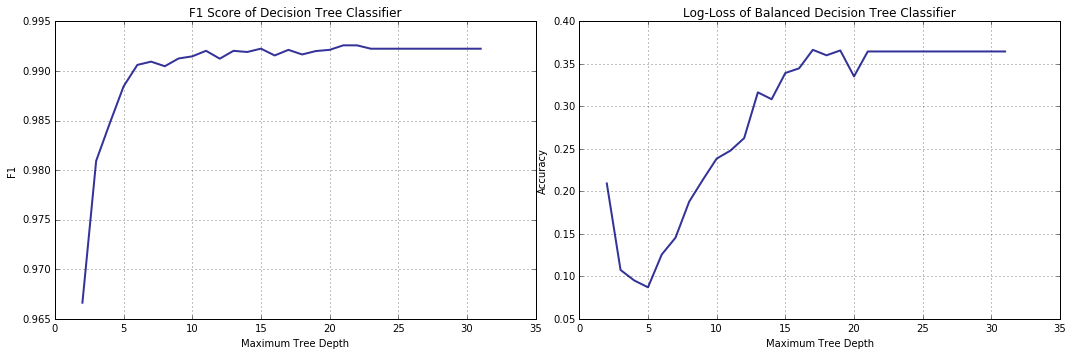
Why did we spend so much time on working out the hypothesis, so clearly wrong? As I have already mentioned, recall is an important measure for malware detection and, as such, merits its own little investigation.
Consider it a red herring if you must…
Hypothesis II: Idiosyncrasies of Log-loss and Decision Trees
So what is actually going on?
To begin with, think how the confidence of a classification algorithm in its predictions changes as the underlying model gains predictive power (i.e the capacity to model larger datasets). In order to answer the question let us plot the proportion of (0, 1) (or (1, 0)) pairs of probabilities returned by predict_proba() method of DecisionTreeClassifier.
1
2
3
tcs, = collect_statistics(cart_depth_lim,
           [ lambda y, p, p0, p1: (np.count_nonzero(p1 == 1.0) +
                                   np.count_nonzero(p0 == 1.0)) / y.shape[0] ] )
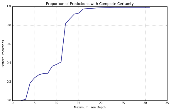
With its depth growing, the decision tree becomes increasingly more confident in its decisions.
However confident we are in our prediction, it can still be wrong. Let us trace the error dynamics by plotting false positive and false negative error rates for the validation set against an increasing tree depth. Among the false predictions, a special place is held by what I call “errors [made] with perfect confidence” where the decision tree estimated the probability of its guess being correct as 1.
1
2
3
4
5
err0, err1, errf0, errf1 = collect_statistics(cart_depth_lim,
    [ lambda y, p, p0, p1: np.sum(p[y_val == 0, 0] == 0.0)/y.shape[0], #false positive with perfect confidence error rate
      lambda y, p, p0, p1: np.sum(p[y_val == 1, 1] == 0.0)/y.shape[0], #false negative with perfect confidence error rate
      lambda y, p, p0, p1: np.sum(p[y_val == 0, 0] < 0.5)/y.shape[0], #false positive error rate
      lambda y, p, p0, p1: np.sum(p[y_val == 1, 1] < 0.5)/y.shape[0] ]) #false negative error rate
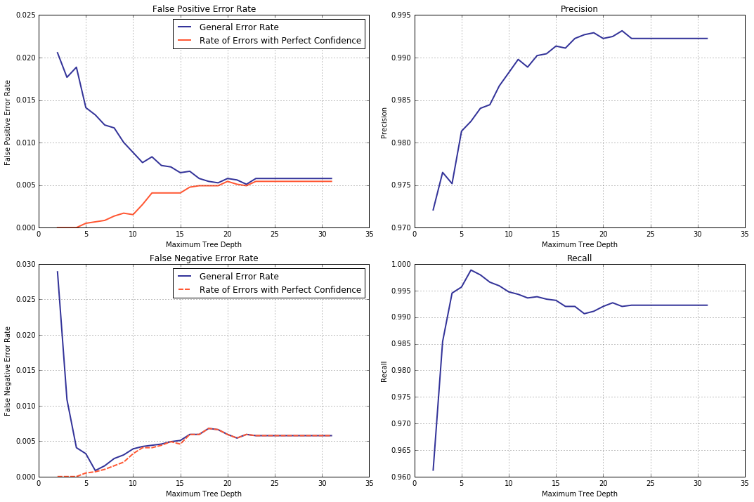
Predictably, trends of false positive and false negative error rates mirror that of precision and recall respectively: namely, FP error rate decreases while precision grows and, FN error rate, dropping at first, shows a gradual increase, which is matched by a rise with subsequent slow decrease in recall. Interesting here is the growth trend displayed by error rates with perfect confidence for both classes. We can, thus, reformulate our earlier conclusion as: with its depth growing, the decision tree becomes increasingly more confident in its blunders. Of course, the mechanism by which it happens is well understood (or rather, can be understood with ease after a quick deliberation).
Remember, a datapoint is classified by being moved down the tree (in accordance with the values of its features and conditions at the tree nodes) until it reaches a leaf. The probability of a datapoint belonging to a particular class is computed as a proportion of the training-set datapoints of the said class that share a leaf with the point being classified.
As a demonstration, we will obtain the probabilities from sklearn, compute the same by hand and then compare the two.
1
2
3
4
5
6
7
8
9
10
11
12
13
14
15
16
17
18
19
p = model_best_recall.predict_proba(X_val)

#index of a datapoint with probabbilities in (0.1, 0.9)
idx = np.where(np.abs(p[:, 0] - 0.5) < 0.4)[0][0]

print("Predicted probabilities of belonging to Benign/Malware classes are", p[idx, :])

leaf_id = model_best_recall.apply(X_val.iloc[idx : idx + 1, :])[0]

print("The Deision Tree places this datapoint to a leaf with an index of", leaf_id)

print("The leaf contains", model_best_recall.tree_.n_node_samples[leaf_id],
      "datapoints, of which",
      model_best_recall.tree_.value[leaf_id][0][0], "are benign and",
      model_best_recall.tree_.value[leaf_id][0][1], "- malware.")

print("The number of benign and malware datapoints in proportion to the total number of datapoints assigned to the leaf:\n",
      model_best_recall.tree_.value[leaf_id][0][0]/model_best_recall.tree_.n_node_samples[leaf_id], "and",
      model_best_recall.tree_.value[leaf_id][0][1]/model_best_recall.tree_.n_node_samples[leaf_id], "respectively.")
1
2
3
4
5
Predicted probabilities of belonging to Benign/Malware classes are [·0.22857143· ¡0.77142857¡]
The Deision Tree places this datapoint to a leaf with an index of 30
The leaf contains 210 datapoints, of which 48.0 are benign and 162.0 - malware.
The number of benign and malware datapoints in proportion to the total number of datapoints assigned to the leaf:
·0.22857142857142856· and ¡0.7714285714285715¡ respectively.
As the tree grows, fewer and fewer nodes contain representatives of both classes and, consequently, more and more datapoints can be classified with perfect confidence, but, of course, this confidence concerns the training data only. It is when the tree has to deal with the data it has not yet seen that “errors with perfect confidence” occur.
If you are not completely convinced, let us for a sample of the same size as before, but taken from the training dataset, plot accuracy, log loss, positive/negative error rates and the same “with perfect confidence” against the limit on tree depth.
1
2
3
4
5
6
7
8
9
10
11
12
13
14
15
from numpy.random import randint

idx = randint(0, X_train.shape[0], X_val.shape[0])

new_X_val = X_train.iloc[idx, :]
new_y_val = y_train.iloc[idx]

t_atrs, t_lsrs, t_err0, t_err1, t_errf0, t_errf1 = collect_statistics(cart_depth_lim,
    [ lambda y, p, p0, p1: accuracy_score(new_y_val, y),
      lambda y, p, p0, p1: log_loss(new_y_val, p),
      lambda y, p, p0, p1: np.sum(p[new_y_val == 0, 0] == 0.0)/y.shape[0],
      lambda y, p, p0, p1: np.sum(p[new_y_val == 1, 1] == 0.0)/y.shape[0],
      lambda y, p, p0, p1: np.sum(p[new_y_val == 0, 0] < 0.5)/y.shape[0],
      lambda y, p, p0, p1: np.sum(p[new_y_val == 1, 1] < 0.5)/y.shape[0] ],
      Xval = new_X_val, yval = new_y_val) # <--- !!!
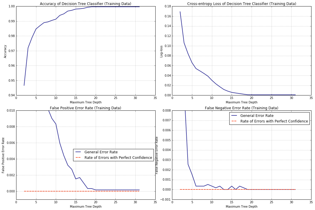
What do we observe? Rates of errors with perfect confidence stay at zero; error rates associated with false positive and false negative predictions, both, decrease and, more to the point, the decrease trend displyed by cross entropy is neatly mirrowed by that for the accuracy.
Obviously, these “overconfident” errors are the culprits in this situation. The sheer audacity of them!..
To see why, recall how log-loss is computed.
\[ll(\mathbb{X}) = \frac{1}{n}\left[\sum_{i=1}^{n} - x^{(i)}_{d+1} \cdot logf(x^{(i)}_1,\ldots,x^{(i)}_d) - (1 - x^{(i)}_{d+1}) \cdot log(1 - f(x^{(i)}_1,\ldots,x^{(i)}_d))\right]\]In case when an error with perfect confidence is comitted, the resulting log-loss will include the term \(1 \cdot log(0)\) and \(log(0)\) is not defined. How does sklearn bypass the problem? Here is an exerpt from the library’s source code:
1
2
3
4
5
6
7
def log_loss(y_true, y_pred, *, eps=1e-15, normalize=True,
             sample_weight=None, labels=None):

    #[...]

    # Clipping
    y_pred = np.clip(y_pred, eps, 1 - eps)
That is, by default, zero probabilities are simply clipped out, being replaced by \(1e-15\). Although far from infinity, the value of \(-log(1e-15) = 34.5388\) is still relatively large (however, keep in mind that its impact is lessened by the fact that log-loss is averaged across all datapoints in the sample). In order to assess the effect it has on the total log-loss of a sample, let us try another substitute for \(log(0)\) – \(0\).
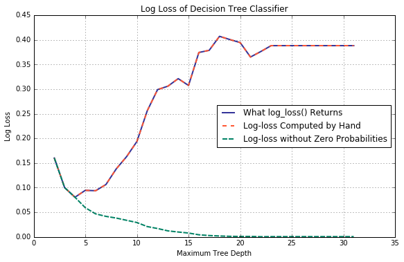
For starters, we will plot partial log-loss computed for each of the classes, Benign and Malware, separately. We will also compute log-loss the sklearn’s way, for comparison.
1
2
3
4
5
6
7
8
9
10
11
12
13
14
15
16
17
18
19
20
21
22
23
24
25
26
27
28
29
30
ll0, ll1, ll = collect_statistics(cart_depth_lim,
    [ lambda y, p, p0, p1: np.sum(-np.log(p0, out = np.zeros_like(p0), #0s by default
                                  where = ( p0 != 0.0 )))/p0.shape[0],
      lambda y, p, p0, p1: np.sum(-np.log(p1, out = np.zeros_like(p1), #0s by default
                                  where = ( p1 != 0.0 )))/p1.shape[0],
      lambda y, p, p0, p1: (np.sum(-np.log(p0, out = np.zeros_like(p0), #0s by default
                                   where = ( p0 != 0.0 ))) +
                            np.sum(-np.log(p1, out = np.zeros_like(p1), #0s by default
                                   where = ( p1 != 0.0 ))))/y.shape[0] ])

#log-loss, the way sklearn computes it
ll_eps = 1e-15

def log_loss_sklean_0(p0):
    p0_cl = np.clip(p0, ll_eps, 1.0 - ll_eps)
    return np.sum(-np.log(p0_cl))/p0.shape[0]

def log_loss_sklean_1(p1):
    p1_cl = np.clip(p1, ll_eps, 1.0 - ll_eps)
    return np.sum(-np.log(p1_cl))/p1.shape[0]

def log_loss_sklean(p0, p1):
    p0_cl = np.clip(p0, ll_eps, 1.0 - ll_eps)
    p1_cl = np.clip(p1, ll_eps, 1.0 - ll_eps)
    return (np.sum(-np.log(p0_cl)) + np.sum(-np.log(p1_cl)))/(p0.shape[0] + p1.shape[0])

llsk0, llsk1, llsk = collect_statistics(cart_depth_lim,
    [ lambda y, p, p0, p1: log_loss_sklean_0(p0),
      lambda y, p, p0, p1: log_loss_sklean_1(p1),
      lambda y, p, p0, p1: log_loss_sklean(p0, p1) ])
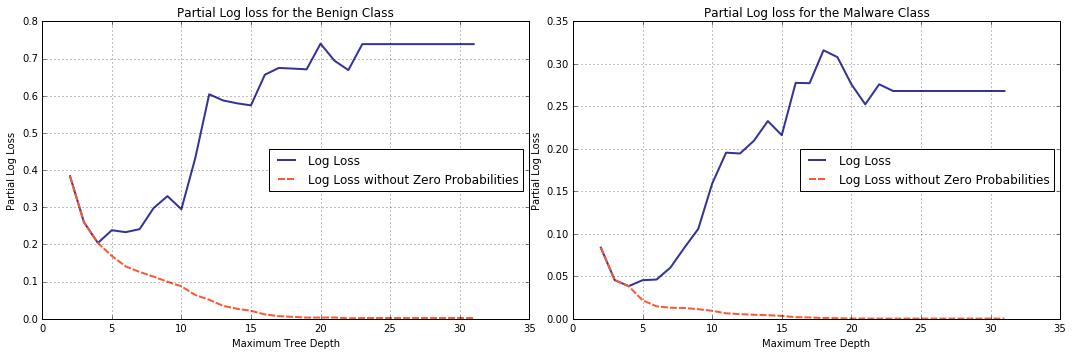
Zero probabilities (and with them, disproportionately large \(log(eps)\)) eliminated, the tendency of cross-entropy metric changes to the opposite and this behaviour is independent of the class, Benign or Malware.
It should come as no surprise that this behaviour is preserved when partial log-losses are combined.
NOTE:
If, for whatever reason, the engineer still insists on using cross entropy as a performance metric, there is a way of mitigating the effect. As you, no doubt, have already guessed, it can be accomplished by increasing the value of paremeter eps passed to log_loss(). Let us plot a family of validation curves for multiple values of eps.
eps1 = 1e-9
eps2 = 1e-5
eps3 = 1e-3
llske1, llske2, llske3 = collect_statistics(cart_depth_lim,
    [ lambda y, p, p0, p1: log_loss(y_val, p, eps = eps1),
      lambda y, p, p0, p1: log_loss(y_val, p, eps = eps2),
      lambda y, p, p0, p1: log_loss(y_val, p, eps = eps3) ])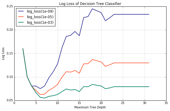
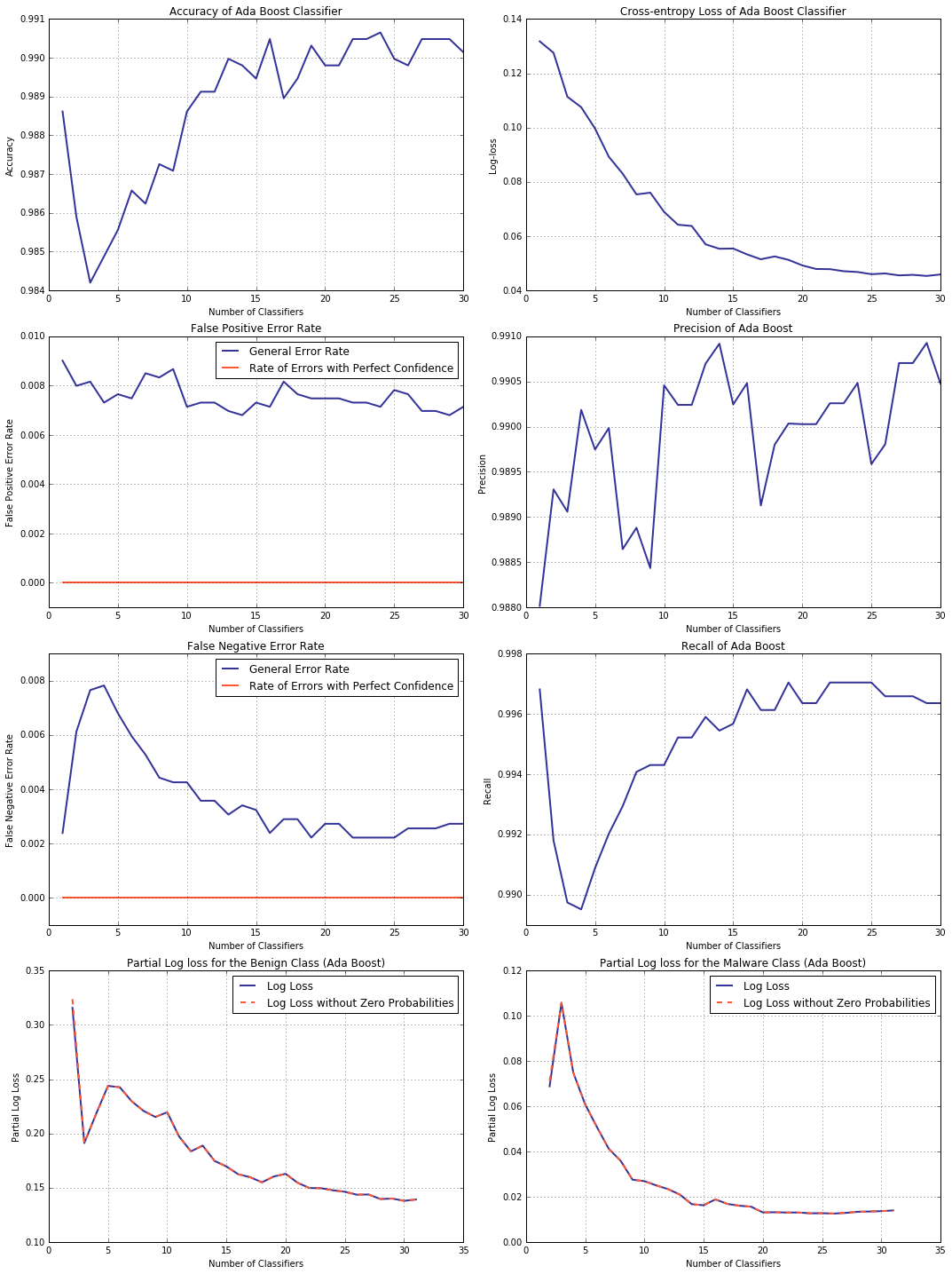
Off the top of one’s head, it is hard to say whether this phenomenon is specific to decision trees and how pervasive it is overall, but, naturally, not all models suffer from this “affliction”. Consider, for example, AdaBoost. For an ensemble classifier, the number of weak learners it employs would be a suitable measure of its complexity, hence this is what we choose to plot the validation curve against.
Examining the plots below, take a note of error rates with perfect confidence staying at zero and decreasing cross-entropy loss.
1
2
3
4
5
6
7
8
9
10
11
12
13
14
15
16
17
18
19
20
21
22
23
24
25
from sklearn.ensemble import AdaBoostClassifier

ada_class_num_lim = lambda i: AdaBoostClassifier(
                                  base_estimator = DecisionTreeClassifier(
                                                       max_depth = 8,
                                                       random_state = rs),
                                  n_estimators = i + 1, random_state = rs)

a_atrs, a_lsrs, a_recs, a_precs, a_err0, a_err1, a_errf0, a_errf1,\\
a_ll0, a_ll1, a_llsk0, a_llsk1 = collect_statistics(
    ada_class_num_lim,
    [ lambda y, p, p0, p1: accuracy_score(y_val, y),
      lambda y, p, p0, p1: log_loss(y_val, p),
      lambda y, p, p0, p1: recall_score(y_val, y),
      lambda y, p, p0, p1: precision_score(y_val, y),
      lambda y, p, p0, p1: np.sum(p[y_val == 0, 0] == 0.0)/y.shape[0],
      lambda y, p, p0, p1: np.sum(p[y_val == 1, 1] == 0.0)/y.shape[0],
      lambda y, p, p0, p1: np.sum(p[y_val == 0, 0] < 0.5)/y.shape[0],
      lambda y, p, p0, p1: np.sum(p[y_val == 1, 1] < 0.5)/y.shape[0],
      lambda y, p, p0, p1: np.sum(-np.log(p0, out = np.zeros_like(p0),
                                  where = ( p0 != 0.0 )))/p0.shape[0],
      lambda y, p, p0, p1: np.sum(-np.log(p1, out = np.zeros_like(p1),
                                  where = ( p1 != 0.0 )))/p1.shape[0],
      lambda y, p, p0, p1: log_loss_sklean_0(p0),
      lambda y, p, p0, p1: log_loss_sklean_1(p1) ])
Conclusion
In the course of this rather extensive (for so straightforward a problem) study we delved into the structure of decision tree predictions and peculiarities of log-loss computation, whilst looking into other topics such as precision and recall scores, decision tree construction and balanced trees along the way. (But this is how research is: one question leads to another and down the rabbit hole you go.)
In the end, an interplay between decreasing error rate and increasing confidence in incorrect predictions (where the latter was overtaking) turned out to be at the core of inconsistency between the accuracy and log-loss trends.
– Ry Auscitte
References
- Andrew Ng, Machine Learning Yearning
- Mauricio Jara, Benign and Malicious PE Files Dataset for Malware Detection
- Virusshare: Repository of malware
- Jason Brownlee, A Gentle Introduction to Cross-Entropy for Machine Learning
- Lei Mao, Cross Entropy, KL Divergence, and Maximum Likelihood Estimation
- Lei Mao, Cross Entropy Loss VS Log Loss VS Sum of Log Loss
- scikit-learn: Machine Learning in Python
- Matt Pietrek, An In-Depth Look into the Win32 Portable Executable File Format, MSDN Magazine (February 2002)