On Computing Expectations of Sample Statistics

Introduction

The subject about to be discussed will, in all probability, seem trivial for the majority of people in statistics and data science. However, it may be considered a source of confusion among undergraduates and “casual mathematicians” such as, say, software engineers who, thanks to AI with machine learning as its flagship having marched in and set up steady camp in the ever-changing world of software, all of a sudden, find themselves reading tons of papers on statistical models.

This post intends to clarify how an expected value of a sample statistic is computed. We, if the reader would care to join the discussion, will focus on a particular kind of statistics – an estimator. I have taken quite a few statistics-related classes, but in none of them were the subtleties involved in the procedure stated explicitly, so writing this post seems worth the effort. This is the way I understand the subject; should you find an issue with my interpretation, I am open for discussion.

Derivation: General Case

Here is the set up. Let \(Z\) be a random variable (it makes no difference whether it is discrete or continuous, 1- or n-dimensional; nevertheless, let us settle on \(Z\) being continuous and scalar in order to simplify the derivation) with the density function \(p(Z \mid \theta = \theta^*)\), where \(\theta^*\) is an unknown parameter. That is, we are dealing with a continuous univariate distribution. \(n\) values are sampled “independently” from the distribution thus forming the sample: \(z_i, \dots, z_n\) with the likelihood of obtaining this sample being \(L(\theta) = \prod_{i=1}^{n}p(Z = z_i \mid \theta)\). Recall that likelihood is a probability of obtaining the data as a function of the distribution parameters.

Our task is to estimate the unknown parameter \(\theta^*\) and what we are looking for is an estimator, i.e. a sample statistic (or, simply put, a function of the sample) that does not depend on \(\theta^*\).

If one were asked for a typical example, the maximum likelihood estimator: \(\widehat{\theta}_{ML} = \argmax_{\theta} L(\theta)\) would be the perfect answer.

A problem of computing an expected value often arises in relation to estimators. For instance, one of the key concepts in estimator evaluation is bias/variance trade-off; to this end, it is necessary to know the bias, which is defined as follows \(bias(\widehat{\theta}) = E[\widehat{\theta}] - \theta^*\). Derived from it are the notions of biased and unbiased estimators with nonzero and zero biases respectively.

How are we to compute the expectation? As it is written now, the estimator is a function of \(n\) realizations of variable \(Z\) and, as such, a constant.

In order to see what is meant by the expectation, we will repeat the sampling process, possibly, indefinitely:

In this context we can talk about \(n\) independent random variables \(Z_1, \dots, Z_n\), identically distributed with the density function \(p(Z_i \mid \theta^{*})\). That is, \(Z_i\) have exactly the same distribution as does \(Z\). Moreover, the estimator is itself can be viewed as a random variable, dependent on \(Z_i\) in accordance with the relation \(\widehat{\Theta} = f(Z_1, \dots, Z_n)\). The distribution of \(\widehat{\Theta}\) is yet to be determined ;-) It depends on \(p\) and \(f\) and should be identified on a case by case basis.

How would you compute an expectation in this interpretation? In my opinion, the procedure below is sound.

This formula can be simplified further. Suppose \(f\) is additively separable, i.e. \(f(Z_1,\ldots,Z_n) = f_1(Z_1) + \dots + f_n(Z_n)\) (a good example of such a relation would be an average when used, say, as an estimator for \(Z\)’s population mean \(\theta^*\): \(f_i(Z_i) = \frac{1}{n} \cdot Z_i\)). Then, by linearity of expectation (\(E[\alpha \cdot X + \beta \cdot Y] = \alpha \cdot E[X] + \beta \cdot E[Y]\)):

By analogy, when \(f\) is separable (w.r.t multiplication), i.e. \(f(Z_1,\dots,Z_n) = f(Z_1) \cdot, \ldots, \cdot f(Z_n)\), from linearity of expectation and mutual independence of \(Z_i\), it follows that

Example: Linear Regression

Applying the theoretical principle or technique one has just learned about to a concrete problem seems a sound idea so this is what we will do next. For a guinea pig, I suggest the least squares estimator that is used to calculate the slope and intercept in simple linear regression. Yes, that ubiquitous linear regression permeating every tutorial, every textbook, every course on statistics or machine learning ever produced. Jokes aside, it would be hard to find a person not (at least at a superficial level) familiar with this fundamental topic so I will not engage in unnecessary lengthy introductions, only reminding the reader that simple linear regression, assuming there is an underlying affine relation between random variables \(X\) and \(Y\): \(Y = \beta_0^* + \beta_1^* \cdot X\) – and \(Y\) is a subject to measurement errors, tries to find the best estimates for \(\beta_0^*\) (intercept) and \(\beta_1^*\) (slope).

The Starting Point

In order to define an estimator, one must first decide on the statistical model to use. We will begin with the following generative model:

(r.v. indices are added to match the explanation of how an estimator expectation is computed)

To put it another way, outcome is a sample of random variable \(Y\), comprised of \(n\) values: \(y_1,\dots y_n\), each generated in the following manner. First, \(X\) is sampled from Exponential distribution parameterized by the parameter \(\lambda\), then, independently of \(X\), a latent random variable \(\mathcal{E}\) is sampled from Normal distribution with zero mean and variance \(\sigma^2\), producing two constants: \(x_i\) and \(\epsilon_i\) as a result. Finally, the value \(y_i\) is obtained from \(x_i\) and \(\epsilon_i\) by applying the formula \(y_i = \beta_0^* + \beta_1^* \cdot x_i + \epsilon_i\). \(\epsilon_i\) is considered a nuisance term, the so-called “noise”. In an ideal setting, there would be a perfect affine relation between \(X\) and \(Y\); in real world, factors of various nature interfere: for example values of \(Y\) may be affected by inaccuracies in measurement, and measurements errors tend to be normal with zero means.

The same procedure may be rewritten in terms of \(X_i\), \(Y_i\), and \(\mathcal{E}_i\) to match our understanding of how an expectation is computed.

Of the variables and parameters mentioned here, we observe \(X\) and \(Y\) only, two sequences of constants \(x_1,\dots,x_n\) and \(y_1,\dots,y_n\) constituting the observations. The objective here is to estimate \(\beta_0^*\) and \(\beta_1^*\). There are multiple ways of doing so; linear regression uses a so-called least squares estimator, which, by the virtue of \(\mathcal{E}\) coming from Gaussian distribution, are identical to a maximum likelihood estimator.

Deriving the Estimators

More so for the sake of completeness than any other reason, I am deriving the estimators in a closed from. The reader may safely skip this section (down to the words “To summarize”) as non-essential.

Linear regression is dealing with a very simple kind of optimization problems, that of minimizing an unconstrained convex objective; in this case, zero gradient is a sufficient optimality condition (see the Convex Optimization textbook by Boyd and Vandenberghe for details).

To summarize:

Note that the numerator and denominator (when multiplied by \(\frac{1}{n-1}\)) of \(\beta_1^{*}\)’s estimator equal: the former to sample covariance \(cov[x, y]\) and the latter to sample variance \(var[x]\), which, themselves, are estimators for population variance and covariance respectively.

Computing Bias

The formulae above may (and should!) be used to compute slopes and intercepts in practice. For theoretical computations, we are free to employ latent variables and unknown distribution parameters. Let us transform estimators’ expressions.

Now let us compute the expectation of estimators in order to check if they are biased. Recall that in order to do that we repeat the sampling process thus giving rise to random variables \(\widehat{\mathcal{B}_0}\) and \(\widehat{\mathcal{B}_1}\).

Taking into account that \(X_i\) and \(\mathcal{E}_i\) are all independent and keeping in mind the property of joint expectations I brought up in one of my earlier posts, the expectation can be easily computed:

What about \(\widehat{\mathcal{B}_0}\)?

By carefully examining the expression above, it is easy to convince oneself that, similar to \(\widehat{\mathcal{B}_1}\), \(E_{X_1,\dots,X_n,\mathcal{E}_1,\dots,\mathcal{E}_n}[\widehat{\mathcal{B}_0}] = \beta^*_0\).

In the context of this generative model, the least squares estimators for \(\widehat{\beta_0}\) and \(\widehat{\beta_1}\) are unbiased.

A Simpler Generative Model

The downsides of the model above will readily become obvious as soon as one embarks on the quest of computing the estimator variance in the name of settling that bias/variance trade-off. Introduced next is a slightly modified model where the task is pleasantly manageable within a short post.

We dispose of the random variable \(X\) and, instead, declare \(n\) constants: \(x_1,\dots,x_n\); they will stay unchanged from sample to sample. This is the model widely adopted across regression-related literature where, when \(x_i\) are multidimensional column vectors, \(\mathbb{X} = [x_1,\dots,x_n]^T\) is referred to as “deterministic design matrix”.

Here is the resulting generative model:

It is easy to check that the expressions for estimators remain the same:

The same can be said about expectations: \(E[\widehat{\mathcal{B}_1}] = \beta_1^*\) and \(E[\widehat{\mathcal{B}_0}] = \beta_0^*\), since \(E_{\mathcal{E}_i}[\mathcal{E}_i] = 0\) as before.

The features being constant, it does not make much sense to describe them in terms of covariance, variance and estimators thereof; for this reason, we define new value \(S_{xy}\) where \(x\) and \(y\) may be sequences of either random variables or deterministic values.

With the new notation in place, we rewrite the equalities derived earlier: \(\widehat{\beta_1} = \frac{S_{xy}}{S_{xx}}\), \(\widehat{\mathcal{B}_1} = \beta_1^* + \frac{S_{x\mathcal{E}}}{S_{xx}}\), \(\widehat{\beta_0} = \overline{y} - \frac{S_{xy}}{S_{xx}} \cdot \overline{x}\), and \(\widehat{\mathcal{B}_0} = \beta_0^* + \overline{\mathcal{E}} - \frac{S_{x\mathcal{E}}}{S_{xx}} \cdot \overline{x}\). Note that \(S_{xx}\) and \(\overline{x}\) are now deterministic and should be treated as constants.

It is time to make good on the promise given at the beginning of this section and calculate the estimators’ variances, which is easily done by applying the rule \(var[\alpha \cdot X + \beta \cdot Y] = \alpha^2 \cdot var[X] + \beta^2 \cdot var[Y] + 2 \cdot \alpha \cdot \beta \cdot cov[X, Y]\) (\(cov[X, Y] = 0\) for independent \(X\) and \(Y\)).

We can extend this result even further. It is a well-known fact that a linear combination of normal random variables (as well as a sum of the same and a constant) is also normally distributed. Now that \(x_i\) are deterministic, by examining the expressions for \(\widehat{\mathcal{B}_0}\) and \(\widehat{\mathcal{B}_1}\) one can easily see that they are nothing more than linear combinations of \(\mathcal{E}_i\) plus deterministic values. Consequently, inferring distribution of these estimators becomes a trivial matter.

To take the discussion further still, consider the following. Now that \(\widehat{\mathcal{B}_0}\) and \(\widehat{\mathcal{B}_1}\) have assumed the shape of proper random variables with distributions and finite first and second moments, they are subject to the law of large numbers and central limit theorem.

Recall that by repeatedly sampling \(X\) and \(\mathcal{E}\) and then computing the intercept and slope as the sample statistics we can form a population of estimators for a fixed value of \(n\): \((\hat{\beta_0}^{(1)}, \hat{\beta_1}^{(1)}), (\hat{\beta_0}^{(2)}, \hat{\beta_1}^{(2)}),\ldots\) (where deterministic \(\hat{\beta_0}^{(i)}\) and \(\hat{\beta_1}^{(i)}\), \(i = \overline{1, \infty}\) are particular realizations of \(\widehat{\mathcal{B}_0}\) and \(\widehat{\mathcal{B}_1}\)).

Of this population, one can take a sample of size \(m\): \((\hat{\beta_0}^{(1)}, \hat{\beta_1}^{(1)}), \ldots, (\hat{\beta_0}^{(m)}, \hat{\beta_1}^{(m)})\) and compute its average (sample or empirical mean) \((\overline{\hat{\beta_0}}, \overline{\hat{\beta_1}}) = \left(\frac{1}{m} \cdot \sum_{i=1}^{m} \hat{\beta_0}^{(i)}, \; \frac{1}{m} \cdot \sum_{i=1}^{m} \hat{\beta_1}^{(i)}\right)\) and empirical variance \((var[\hat{\beta_0}], var[\hat{\beta_1}]) = \left(\frac{1}{m-1} \cdot \sum_{i=1}^{m} (\hat{\beta_0}^{(i)} - \overline{\hat{\beta_0}})^2,\; \frac{1}{m-1} \cdot \sum_{i=1}^{m} (\hat{\beta_1}^{(i)} - \overline{\hat{\beta_1}})^2 \right)\). Following exactly the same line of reasoning as we did for the estimators, we can replicate this experiment indefinitely (i.e. take infinitely many samples of size \(m\) from the population) and raise the empirical mean and variance to the “rank” of random variables: \(\overline{\widehat{\mathcal{B}_0}}\), \(\overline{\widehat{\mathcal{B}_1}}\), \(\widehat{var[\widehat{\mathcal{B}_0}]}\), and \(\widehat{var[\widehat{\mathcal{B}_1}]}\). It works for any sample statistic: be it an estimator, an average or a sample variance. Among the statistics, average, however, holds a special place thanks to the famous law of large numbers.

Imagine now that not only do we replicate the experiment, but also increase the sample size \(m\) each time: \(m = m_0, m_0 + 1, m_0 + 2, \dots\). The law of large numbers (LLN) predicts that as \(m\) goes to infinity, the average (sample mean) converges to the expectation (population mean), i.e.

One of LLN’s corollaries states that sample variance of a random variable also converges (almost surely and in probability) to its theoretical counterpart, population variance. Remember that sample variances of estimates for \(\beta_0^*\) and \(\beta_1^*\) can be treated as random variables \((\widehat{var[\widehat{\mathcal{B}_1}]}\) and \(\widehat{var[\widehat{\mathcal{B}_1}]}\)); taking infinitely many samples with increasing sample \(m\), we obtain an infinite sequence of random variables that converges to the population variance. On the other hand, sample variance is an estimator of population variance (hence the hats above \(var[]\)), therefore the estimator converges to the estimated value.

Finally, let us apply the central limit theorem (CLT) to \(\widehat{\mathcal{B}_0}\) and \(\widehat{\mathcal{B}_1}\):

A happy consequence of CLT consists in that we can now approximate the distribution of \(\overline{\widehat{\mathcal{B}_i}}\) for sufficiently large \(m\) (usually, \(m \ge 30\) is named as the threshold).

An observant reader will have noticed that \(\widehat{\mathcal{B}_i}\) had already been established to come from Gaussian distribution. Given an average is nothing more than a scaled sum of variables (and, therefore, must also be Gaussian), the CLT result seems excessive. However, unlike the earlier inference, this one did not involve restrictions on the distribution of \(\mathcal{E}\) or \(Y\). Diving a little deeper, one concludes that even with no such restrictions in place, \(\widehat{\mathcal{B}_i}\) will still likely to look normal since expressions for the slope and intercept can be reduced to sums of scaled identically distributed variables (\(Y_i\)) and these sums tend to be normally distributed (provided the number of datapoints \(n\) is large).

In a nutshell, \(\overline{\widehat{\mathcal{B}_i}}\) follow Normal distribution in the limit, but under additional assumptions, stronger statements can be made. Below is progression from the strongest to the weakest statement:

• \(\widehat{\mathcal{B}_i}\) (and \(\overline{\widehat{\mathcal{B}_i}}\) by extension) are normally distributed if the noise is.
• \(\widehat{\mathcal{B}_i}\) (and \(\overline{\widehat{\mathcal{B}_i}}\) by extension) are approximately normally distributed (irrespective of noise distribution) if \(n\) is large enough.
• \(\overline{\widehat{\mathcal{B}_i}}\) is normally distributed in the limit \(m \rightarrow \infty\) irrespective of noise distribution or sample sizes.

So, what have we been up to (for the whole ten A4 pages)? From a generative model of our choosing, we obtained a sample of \(n\) random values and used it to compute a slope and an intercept. What we had computed were sample statistics that were also estimators for coefficients in an assumed underlying affine relation between variables and/or deterministic values within the framework of the generative model. The observation that infinitely many such samples might be taken, thus resulting in infinitely many slopes and intercepts, led us to the conclusion that the estimated values (and any sample statistics, overall) were random variables as well. We proceeded by inferring the distribution linear regression coefficients followed. Then, the estimates being random, it was possible to sample from their distributions, producing samples of size \(m\), and compute some kind of statistic. This time an average was chosen. By analogy, the average must be a random variable and, following in our own footsteps, we figured out what its distribution was…

I could have gone on forever with this recursive process of turning sample statistics into random variables with subsequent inference of their distributions in order to produce more samples and compute new statistics (along the way, testing how many hats and bars latex could stack on top of each other before the rendering engine collapsed) and, no doubt, it would have made for a fascinating endeavor. But eventually I would have run our of food and grew uncomfortable. So I am choosing to stop here, my sincere hope being that this little exercise allowed the reader to get a good grasp on the nature of sample statistics (and estimators, in particular).

Illustrative Experiments

A special kind of delight lies in seeing the theoretical results (above all, those one has come up with on her own) work in practice. This section is for those of my readers who like to code. We will conduct experiments illustrating unbiasedness of linear regression estimators and confirm that the statistics mentioned in the “theoretical” part of the post, being random in nature, indeed, come from the distributions we deduced.

I will post the key code fragments for the purposes of clarity, whereas tedious plotting-related functionality will be omitted. Not to worry: an accompanying R notebook containing the code in all its entirety can be found here or here.

Generative Models Implementation

Let us begin by defining the functions that generate random samples and compute linear regression coefficients. It may prove illuminating to run both models – with random and deterministic features (explanation/design variables) side by side with the view of comparing the rates of convergence and other effects. Since multiple generative models are supported and parameters required to specify these models differ, we will use R’s environments (passed as a parameter named “varargs”) in order to implement the variable number of arguments.

1
2
3
4
5
6
7
8
9
10
11
12
13
14
15
16
17
18
19
20
21
22
23
24
25
26
27
28
29
30
31
32
33
34
35
36
37
38
39
40
41
42
43
44
45
46
47
48
49
50
51
52
53
54
55
56
57
58
59
library(rlang)

Sxy <- function(x, y) {
    sum(x * y) - mean(x) * sum(y)
}

gaussian_noise <- function(n, varargs) {
    stopifnot(env_has(varargs, "noise_sd"))
    rnorm(n, mean = 0, sd = varargs$noise_sd)
}

#Explanation variable for the 2-Step generative model
exponential_feature <- function(n, varargs) {
    stopifnot(env_has(varargs, "FeatureParam"))
    rexp(n, varargs$FeatureParam)
}

#Explanation variable for the 1-Step generative model
deterministic_feature <- function(n, varargs) {
    stopifnot(env_has(varargs, "XSource"))
    varargs$XSource[1:n]
}

#Replicates computing least squares estimates for coefficients of 
#simple linear regression based on a n-sized sample m times
sample_beta_estimator <- function(m, n, beta0, beta1, varargs) {

    beta_hats <- data.frame()

    for (i in 1:m) {

        #generating the data
        X <- varargs$gen_feature(n, varargs)
        eps <- varargs$gen_noise(n, varargs)
        Y <- beta0 + beta1 * X + eps

        #computing the estimators
        Y_bar <- mean(Y)
        X_bar <- mean(X)
        beta_hat <- c(Y_bar - (Sxy(X, Y) / Sxy(X, X)) * X_bar, Sxy(X, Y) / Sxy(X, X))

        beta_hats <- rbind(beta_hats, beta_hat)
    }

    beta_hats
}

#Computes empirical mean and variance of estimated linear regression
#coefficients averaged over m runs, each involving calculation of the 
#least squares estimates for a sample of size n
moments_of_beta_estimator <- function(m, n, beta0, beta1, varargs) {

    beta_hats <- sample_beta_estimator(m, n, beta0, beta1, varargs)
 
    beta_hat_bar <- c( mean(beta_hats[, 1]), mean(beta_hats[, 2]) )
    beta_hat_var <- c( var(beta_hats[, 1]), var(beta_hats[, 2]) )

    c(beta_hat_bar, beta_hat_var)
}

The code should speak for itself: sample_beta_estimator() returns an m-sized sample of slopes and intercepts while moments_of_beta_estimator(), in addition, computes mean and variance of that sample.

Next we define the latent distribution parameters for random constituents of the model; where the data is deterministic, a vector of the maximum necessary length n_max is generated in advance and used unchanged throughout all the computations.

1
2
3
4
5
6
7
8
9
10
11
12
13
14
15
16
#Distribution parameter for the explanatory variable  
lambda <- 2
#Standard deviation for the Gaussian noise
sigma <- 3
#True (latent) values for regression coefficients
beta_star <- c(5.5, 2.2)
#Deterministic X for the 1-Step model (not treated as a random variable)
Xfull <- rexp(n_max, lambda) 

#Parameters for the 2-Step generative model
env_2st <- env(gen_noise = gaussian_noise, noise_sd = sigma, 
               gen_feature = exponential_feature, FeatureParam = lambda)

#Parameters for the 1-Step generative model
env_1st <- env(gen_noise = gaussian_noise, noise_sd = sigma, 
               gen_feature = deterministic_feature, XSource = Xfull)

Visualizing Consistency of the Estimators

One would expect the absence of bias to be visualized first as it was the fist property considered. Perplexing, therefore, the reader may find the decision to begin with something we have not touched upon at all. What can I say? The world is a mysterious place, full of surprises and ready to throw you into a stupor of incredulity any moment.

So we begin by demonstrating that the least squares estimators are consistent, which is accomplished in an experiment very similar to that intended to show the absence of bias. It is important to recognize the difference.

An estimator \(\hat{\theta}\) for the true distribution parameter \(\theta^*\) computed as a sample statistic over a sample of size \(n\) is called consistent if \(\lim_{n \rightarrow \infty}{\hat{\theta}} = \theta^*\). Again, notions of weak and strong consistency are defined depending on the type of convergence involved and, as before, in case of linear regression, both apply. In order to visualize consistency, we will plot the estimated coefficient: \(\beta_0\) or \(\beta_1\) – alongside its true value for an increasing number of datapoints \(n\). The sequence of sample sizes will be non-linear with the greater density of points near small \(n\)s, where we expect greater variability in the estimator’s values; it is meant to reduce the running time.

1
2
3
4
5
6
7
8
9
10
11
12
13
14
15
16
17
18
19
20
21
22
#Computes beta0 and beta1 estimates for gradually increasing sample sizes 
#in order to show consistency of the estimator
collect_data_for_consistency_demo <- function(varargs) {

    n_seq <- c(seq(100, 999, 100), 
               seq(1000, m_max_nobias, 500), 
               seq(m_max_nobias + 1, n_max, 1000))

    beta_hats <- data.frame()
    for (n in n_seq) {
        #m == 1, the estimates are computed once only for each n
        beta_hats <- rbind(beta_hats, 
            c(n, sample_beta_estimator(1, n, beta_star[1], beta_star[2], varargs)))
    }

    names(beta_hats) <- c("n", "beta0", "beta1")

    beta_hats
}

beta_hats_2step <- collect_data_for_consistency_demo(env_2st)
beta_hats_1step <- collect_data_for_consistency_demo(env_1st)

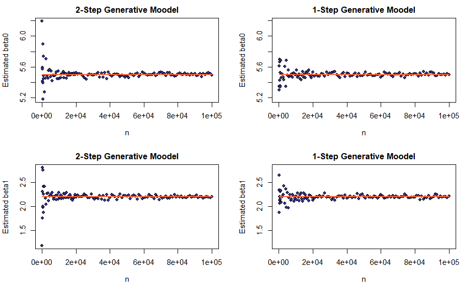
Although not proven here, judging by the plot, the consistency claim seems to hold.

Visualizing Unbiasedness of the Estimators

Now let us proceed to visualizing the absence of bias. Here, the experiment setup is slightly more complicated. This time the number of datapoints is kept fixed at n_fixed and the sampling procedure is repeated m times (and not once only as in the previous experiment). For each sample, we compute the LS estimators as statistics of that sample and then average the estimated values over m runs thereby obtaining the estimators’ empirical means and variances. By the law of large numbers, average and sample variance of a random variable should go to its expectation and population variance respectively as the sample size goes to infinity. Keep in mind, it is \(m\) that goes to infinity while \(n\) remains fixed!

Least squares estimators for linear regression coefficients are unbiased, therefore their expectations must be equal to the true values of the coefficients in the underlying affine relation. Consequently, as m increases, we should observe average estimated values for a coefficient concentrate around its true value.

As before, a non-linear sequence of m is used, but in order to keep the running time within reasonable limits we have to limit the number of experiments.

1
2
3
4
5
6
7
8
9
10
11
12
13
14
15
16
17
18
19
20
21
#Computes sample mean and variance for a sequence of m-sized samples of estimated 
#beta0 and beta1, each, in turn, computed based on a n_fixed-sized sample of X and Y. 
collect_data_for_bias_demo <- function(varargs) {

    m_seq <- c(seq(100, 999, 100), seq(1000, m_max_nobias, 500))

    beta_hat_means <- data.frame()
    for (m in m_seq) {
        beta_hat_means <- rbind(beta_hat_means, 
            c(m, moments_of_beta_estimator(m, n_fixed, beta_star[1], 
                                           beta_star[2], varargs)))
    }

    names(beta_hat_means) <- c("m", "mean_beta0", "mean_beta1", 
                               "var_beta0", "var_beta1")

    beta_hat_means
}

beta_hat_means_2step <- collect_data_for_bias_demo(env_2st)
beta_hat_means_1step <- collect_data_for_bias_demo(env_1st)

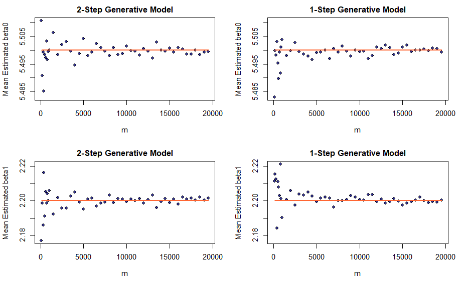
Well, the means of estimated coefficients do converge, but, to our disappointment, the convergence appears less pronounced. The next section will explain what is going on.

On Convergence Rates

Comparing the convergence plots illustrating consistency and unbiasedness properties of the LS estimators, one may falsely conclude that in the case of consistency, the observed values converge to the true ones faster. However, it is only an illusion created by the difference in the restrictions we have put on the maximum values of \(n\) and \(m\) and resulting difference in scale.

In order to estimate the actual convergence rates, we combine data points for the same values of \(n\) and \(m\) on a single figure (which, I will be the first one to admit, is a bit like comparing apples to oranges). In particular, an absolute difference between the estimated and true value of the coefficient \(\beta_1\) in the context of 1-Step model will be plotted.

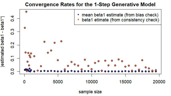
Contrary to our previous observation, an average converges faster than an individual estimator. It may also be helpful to consider the difference in variances of the estimated values \(\hat{\beta_1}\) and the same, averaged over \(m\) samples, while keeping in mind that smaller variances translate into faster convergence rates. Recall that \(var[\frac{1}{m} \cdot \sum_{i=1}^{m} Z_m] = \frac{1}{m^2} \cdot \sum_{i=1}^{m} var[Z_m]\).

1
2
3
4
5
6
7
8
9
10
11
12
13
14
15
16
17
var_beta_0 <- function(noise_sd, x) {
    noise_sd^2 * (1/length(x) + (mean(x)^2)/Sxy(x, x))
}

var_beta_1 <- function(noise_sd, x) {
    noise_sd^2 / Sxy(x, x)
}

vars_cons <- vector()
vars_bias <- vector()
#skip the first few extra large variances to obtain a better-scaled plot
first_n <- n_min 
for (num in first_n:lim_n) {
    vars_cons <- c(vars_cons, var_beta_1(sigma, Xfull[1:beta_hats_1step$n[num]]))
    vars_bias <- c(vars_bias, 
                   var_beta_1(sigma, Xfull[1:n_fixed]) / beta_hat_means_1step$m[num])
}

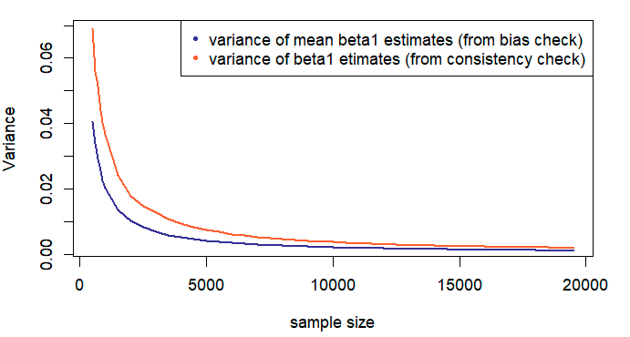
Visualizing the LLN Results for Variances

Similar to the means, sample variances of the estimators go to the respective population variances as the number of runs (\(m\)) increases. Apart from the fact that we derived expressions for population variances in the setting of the 1-Step Model only, the plots are constructed similar to the ones for means.

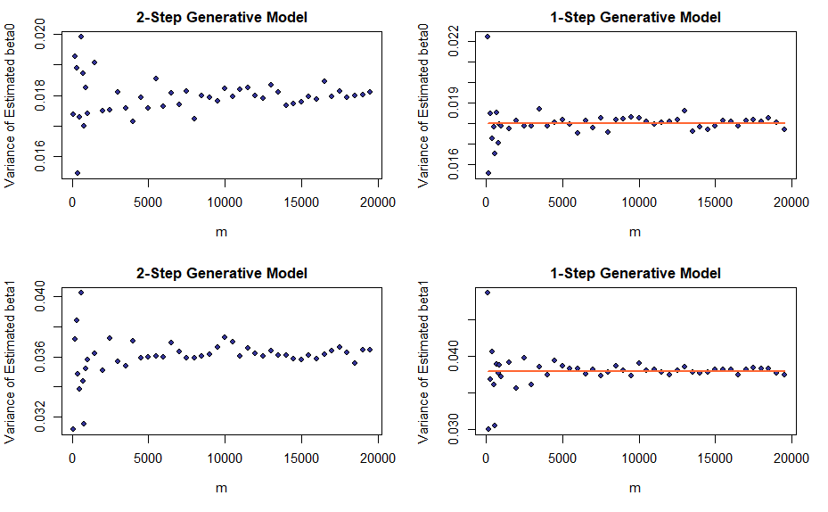
Distribution of the Estimated Values

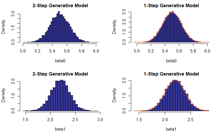
In the setting of the 1-Step Model, the estimated values for the linear regression coefficients have been shown to be normally distributed with means \((\beta_0^*, \beta_1^*)\) and variances dependent on \(X\) and standard deviation of noise. We did attempt achieving equivalent results for the 2-Step generative model.

Akin to the previous experiment, the population of slopes and intercepts is sampled \(m\) times, with the key difference being that \(m\) remains fixed rather than coming from an increasing sequence of values; the outcome is a collection of \(\hat{\beta_0}\) and \(\hat{\beta_1}\), \(m\) values each (no averages are computed). Then we construct histograms of the estimated values and see how well they match the theoretical probability density functions (PDFs).

1
2
3
4
5
6
7
8
9
10
11
12
13
14
15
16
m <- 10000

#collecting data for the 2-step model 
beta_hats_2step_h <- sample_beta_estimator(m, n_fixed, 
                                           beta_star[1], beta_star[2], 
                                           env_2st)

#collecting data for the 1-step model
beta_hats_1step_h <- sample_beta_estimator(m, n_fixed, 
                                           beta_star[1], beta_star[2], 
                                           env_1st)
#computing theoretical beta PDFs for the 1-step model
beta0_pdf <- normal_curve(beta_hats_1step_h[,1], beta_star[1], 
                          sqrt(var_beta_0(sigma, Xfull[1:n_fixed])))
beta1_pdf <- normal_curve(beta_hats_1step_h[,2], beta_star[2], 
                          sqrt(var_beta_1(sigma, Xfull[1:n_fixed])))

Distribution of the Estimator’s Means

Not only do we know how the estimated \(\beta_i\) values are distributed, central limit theorem also gives us the information concerning distribution of their means (in the limit). Let us construct histograms for various values of \(m\) in an effort to confirm that the distribution of \(\frac{\sqrt{m} \cdot (\overline{\widehat{\mathcal{B}_i}} - \beta_i^*)}{\sqrt{var[\widehat{\mathcal{B}_i}]}}\), indeed, approaches standard normal as \(m\) increases. In order to achieve this, we must wrap our data collection procedure in another loop, this time over \(k\).

The demonstration will be limited to the 1-step generative model.

1
2
3
4
5
6
7
8
9
10
11
12
13
14
15
16
17
18
19
20
21
22
23
24
25
26
27
k_max <- 2000
m_seq <- c(1, 10, 1000)

#Collects k samples of mean estimated values for the linear regression coefficients
#along with respective sample variances.
#Each estimated value is computed for a n-sized sample of X and Y; then an average
#and sample variance are calculated over m such values.
replicate_average_estimator <- function(m, n, k, varargs) {
	
    bh <- data.frame()

    for (i in 1:k) {
        bh <- rbind(bh, c(moments_of_beta_estimator(m, n, beta_star[1], 
                                                    beta_star[2], varargs)))
    }

    names(bh) <- c("mean_beta0", "mean_beta1", "var_beta0", "var_beta1")
    bh
}

#running replicate_average_estimator for various values of m 
#(given by the sequence m_seq)
beta_hat_means_1step_cm <- lapply(m_seq, replicate_average_estimator, 
                                  n_min, k_max, env_1st)
#theoretical variances of estimated linear regression coefficients
beta_vars_cm <- c(var_beta_0(sigma, Xfull[1:n_min]), 
                  var_beta_1(sigma, Xfull[1:n_min]))

Notice that unlike in the previous experiment, where we visualized the distribution of estimated values themselves and not their means, here the function moments_of_beta_estimator() is called instead of sample_beta_estimator().

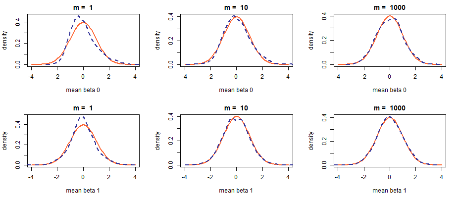
For convenience, we will plot the PDFs interpolated from histograms along with a PDF of the standard normal distribution for various values of \(m\). What we are hoping to see is the reconstructed PDF gradually shaping into that of \(\mathcal{N}(0, 1)\).

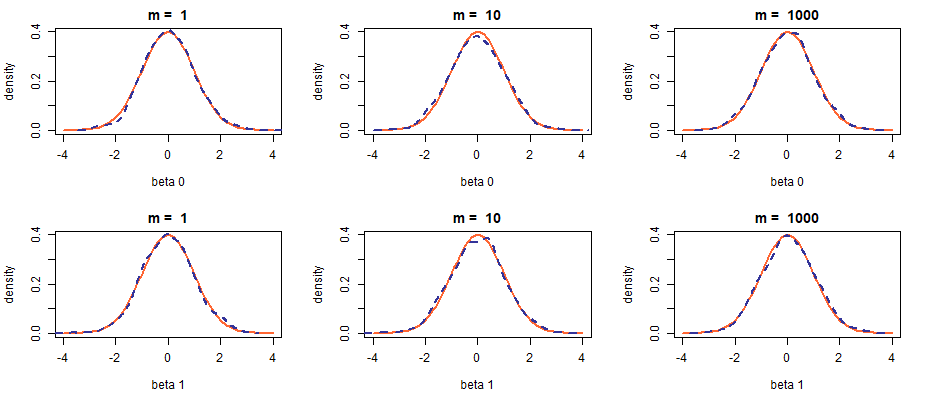
The plots do not seem to change drastically with an increase in sample size and the effect of convergence in distribution is not clearly visible. It should not be. When the noise is Gaussian, the estimated values themselves are already normally distributed and so are their averages, even for very small \(m\). Let us try using another distribution to generate the noise.

Distribution of Estimator’s Means (Beta Noise)

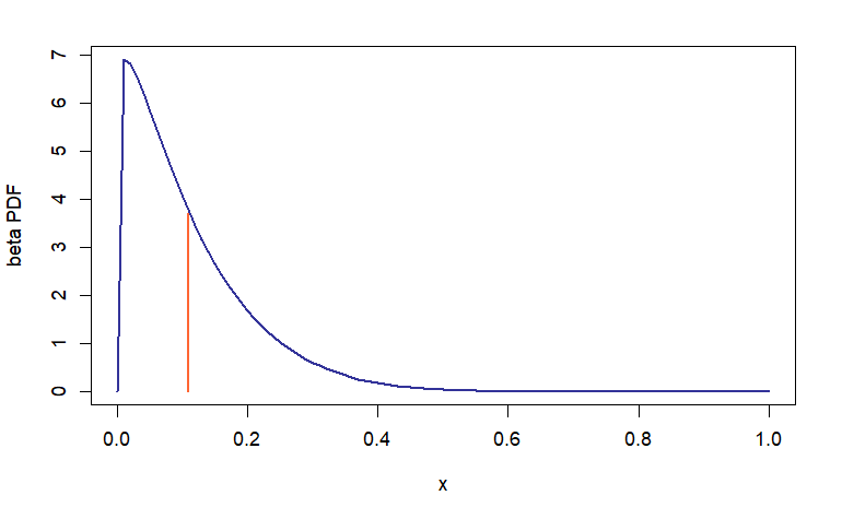
Which of the known distributions can we choose? The possibilities are numerous while restrictions are not: the distribution of choice must have finite variance and zero expectation (\(E[\mathcal{E}] = 0\) is used in many of our derivations). Why not Beta distribution shifted to the left by the value of its mean?

1
2
3
4
5
6
7
8
9
10
11
12
13
14
15
16
17
18
19
20
21
alpha <- 1.1
beta <- 9

#samples n values from beta distribution
beta_noise <- function(n, varargs) {
    stopifnot(env_has(varargs, "alpha"))
    stopifnot(env_has(varargs, "beta"))
    rbeta(n, varargs$alpha, varargs$beta) - 
             varargs$alpha / (varargs$alpha + varargs$beta)
}

env_1st_bn <- env(gen_noise = beta_noise, alpha = alpha, beta = beta, 
                  gen_feature = deterministic_feature, XSource = Xfull)

beta_hat_means_1step_bncm <- lapply(m_seq, replicate_average_estimator, 
                                    n_min, k_max, env_1st_bn)

#standard deviation of Beta distribution
bn_sd <- sqrt((alpha * beta)/(alpha + beta + 1.0)) * (1.0/(alpha + beta))
beta_vars_bncm <- c(var_beta_0(bn_sd, Xfull[1:n_min]), 
                    var_beta_1(bn_sd, Xfull[1:n_min]))

This is when the developer may congratulate herself on making a foresighted design decision. Look how easy it is to replace the existing Gaussian noise distribution with any one of our choosing, but I digress. An interesting feature of Beta distribution with these particular parameters is its asymmetry relative to the mean (one of the reasons why I picked it), a property that should be reflected (one way or another) in the resulting density shape of \(\hat{\beta_i}\).

Software developers who make foresighted design decisions tend to exhibit a fair degree of clairvoyance in other realms too (he-he) and I can tell you right away that changing noise to non-Gaussian will not be enough. A cursory glance at the formula for computing the \(\hat{\beta_1}\) estimator leads us to the conclusion that the estimated values may still be roughly normally distributed (even if the noise is not Gaussian) when \(n\) is large enough. For this reason, n_min (set to 5) is used in place of n_fixed (lines 16, 20, and 21 in the code chunk above).

The change of distribution achieves the desired effect; however, notice how quickly the mean estimators “normalize”: at \(m = 10\) the skew is barely discernible. It has been eons since I learned about LLN and CLT and it is comforting to know they still work ;-)

Conclusion

Prompted by a mundane task of computing an estimator’s expectation arising as a part of the bias/variance tradeoff analysis, we got an opportunity to take a deeper dive into the nature of sample statistics and, hopefully, emerged with a slightly deeper understanding of the subject.

– Ry Auscitte

References

1. Stephen Boyd and Lieven Vandenberghe (2004), Convex optimization, Cambridge university press
2. Javed Hussain, Lecture 16 (Part 1): Weak vs Strong law of large numbers (intuition, differences and similarities), Introduction to Mathematical Probability, Sukkur IBA University
3. Robert Gallager, 6.262 Discrete Stochastic Processes, Spring 2011, MIT
4. Robert Gallager, Renewals and the Strong Law of Large Numbers, MIT, Discrete Stochastic Processes (2011), MIT
5. Felix Pahl, Sample Variance Converges Almost Surely
6. Douglas Shafer and Zhiyi Zhang, The Sampling Distribution of the Sample Mean, Beginning Statistics (2012)
7. Ry Auscitte, A Quick Note: Some «Trivia» about Joint Expectations (2022), Notes of an Innocent Bystander (with a Chainsaw in Hand)