A Universal Law of CheckSum Values Distribution in PE Files
Introduction
Ubiquity of various binary patching techniques, of which compression, encryption, and obfuscation performed by PE packers are particularly common forms, in the world of malware led to the checksum stored in PE’s IMAGE_OPTIONAL_HEADER playing the role, more significant than initially intended. Michael Lester, the author of Executable Features Series on Practical Security Analytics goes as far as to claim the PE checksum to be “the single greatest stand-alone indicator of malware […] even more so than digital signatures” in his blog post.
The CheckSum field is intended to aid in ensuring integrity of binary files since the latter might get corrupted while transmitted over a network or in storage. The reader might be interested to know that for user-mode applications, the checksum correctness is not actually enforced by Windows. It is only the modules mapped into address spaces of critical processes, drivers, and dlls loaded at boot time that are bestowed with this kind of assiduous attention. One can launch an exe with invalid checksum without so much as a notice from the OS. What is more, by default (unless one compiles a driver), Microsoft’s vc toolchain (tested on ver. 14) does not even compute the checksum, leaving the field initialized to zero. A developer wishing to obtain a binary with the correct checksum should pass a /RELEASE key to the linker (details are in the documentation, here and here).
No wonder that every now and then one comes across an absolutely innocuous binary with an invalid checksum; yet, due to the specifics of the tools used, it is malware modules that are especially prone to checksum errors. According to Michael Lester,
83% of malware had invalid checksums
90% of legitimate files had valid checksums
Based on the above, prioritizing binaries with incorrect checksums when looking for the culprit covertly disrupting the system’s operation suggests itself as a viable strategy. However, a question of whether this statistics is based on a representative sample and how it applies to the population in general arises and this is the question this post attempts to (partially!) answer.
As far as malware is concerned, I can do no more than test the PE binaries in publicly-accessible malware databases for the validity of their checksums. There is little doubt that these numbers have already been incorporated into the result presented by the Practical Security Analytics. But what if I take a typical system, where the majority of modules are benign? Will the 90/10 ratio hold? Here is the plan: I will collect the checksum statistics on my Windows laptop (along with some additional information about the binaries), examine the checksum distribution and see if it leads to illuminating insights. Of course, the results will be inconclusive due to the data shortage (it is only one system, after all), but, nonetheless, it seems a fun project to do. This is the endeavor the reader is invited to join.
Collecting the Data
The task at hand is straightforward enough: enumerate all the PE files in the system, recording if their checksums are correct or not as we go. The easiest way of accomplishing it is with the help of Ero Carrera’s pefile; implemented therein is the PE::verify_checksum() function which might prove to be of assistance. But let us abstain from taking the easy road and instead implement a solution that can be used on Python-less systems.
My implementation is available on github; it is a small utility written in old-style C++ and buildable with the toolchain that comes with MS Visual C++ or Windows SDK (or whatever it is called now; Microsoft does its best to break the monotony of software developers’ boring lives by rearranging and renaming the SDK every once in a while). Having compiled the utility, one can then collect the statistics from a variety of systems (which the reader is insistently encouraged to do, as our results, when combined, will carry at least some degree of credibility).
The utility being rather simple, I will not post the source code in its entirety or provide a detailed explanation here; however, should one take interest in the way checksums are validated, the lines to look for are these two:
1
2
3
DWORD dwHeaderSum = 0, dwCheckSum = 0;
IMAGE_NT_HEADERS*  pHdrs = CheckSumMappedFile(pMap, ffd.nFileSizeLow,
                                              &dwHeaderSum, &dwCheckSum);
I am using CheckSumMappedFile() from the ImageHlp API; it returns the value stored in the PE header (dwHeaderSum) and the checksum it computes based on the file contents (dwCheckSum); so the checksum validation becomes a simple matter of comparing the two. The only difficulty facing us here is that CheckSumMappedFile() requires the binary file to be mapped into the process’ address space, which explains the appearance of FileMaps, a structure that encapsulates file mappings and avoids resource leaks by automatically releasing handles in its destructor.
One can think of CheckSum as a hash function of the file contents and record stats in terms of collision counts for each encountered value of checksum (rather than collecting <file, checksum> pairs for individual files), thereby saving space, and this is what I have chosen to do (see ChecksumStats::AddGoodCheckSum() and ChecksumStats::AddBadCheckSum()). As a consequence, the utility creates two csv files, one containing collision counts for valid and another – for invalid – checksums.
In order to gain valuable insights and, possibly, lay foundation for future projects, let us collect additional data. As mentioned earlier, without the /RELEASE linker option, PE’s CheckSum field stays initialized to zero. What if we come across a checksum that is both, invalid and non-zero? There are three possible explanations: either the linker employed to build the binary computes the checksums incorrectly, the file has been patched post-linking or tampered with at a binary level by a third party. The latter two are particularly difficult to tell apart; as for the first one, a large portion of modern software is built with Microsoft’s toolchain, which, first of all, must be computing checksums correctly, and, second of all, is easily identifiable by the so-called Rich header embedded into the resulting PE file. Next, the (nearly) ironclad proof of third-party tampering is a damaged digest (though it does not always work as we will see later), so recording if the binary is digitally signed and the signature checks appears to be a good idea.
1
2
3
4
5
6
void ChecksumStats::AddBadCheckSumDetailedRecord(int nFields, ...);
//[...]
pStats->AddBadCheckSumDetailedRecord(3, //number of arguments that follow
    sFullPath,
    VerifySignature(sFullPath.c_str(), mps.GetFileHandle(pMap)),
    String(ContainsRichHeader(pMap) ? TEXT("Rich Header") : TEXT("No Rich")));
Of course, the collected information is not enough to distinguish tampering with malicious purposes from the legitimate modifications; this is why ChecksumStats::AddBadCheckSumDetailedRecord(int nFields, ...) is designed to accept a variable number of arguments. For example, one might add packers detector identifying the packer(s) used to meddle with the binary. The possibilities are endless ;-)
Exploring the Data
At a Glance
Running (with appropriate privileges) the utility on my laptop produces the output below.
1
2
> CheckSumStats.exe C: good.csv bad.csv baddetails.csv
Found 64121 binaries: 56652 with correct checksum and 7469 with incorrect
A bit of tinkering with csv files gives us extended output:
1
2
3
4
## Out of 64121 binaries, there are
##    * 56652 with valid checksums (88.35%) and
##    * 7469 with malformed checksums (11.65%).
## Of the latter, 7135(95.53%) have zero checksum.
I do not keep malware collections on the laptop in question; even if there are some malicious (“malicious” as defined by anti-malware products; although should one run our stats-collecting utility overnight without enabling the “No auto-restart with logged-on users for scheduled automatic updates” policy first, one might end up feeling compelled to challenge this definition) binaries there, they are not numerous, hence the body of tested software may be qualified as (mostly) legitimate. Thus, 11.65% of legitimate binaries in the system have invalid checksums. Surprisingly, the number is, though not exactly the declared 10%, but close enough!
There must be a universal law of PE checksum distribution, according to which an equilibrium is reached at the 90/10 ratio of valid to invalid checksums; any perturbation initiates a process of checksum update gradually reestablishing the equilibrium. Jokes aside, remarkable as it is, the result may still be coincidental rather than illustrative of the general trend. On the other hand, it may reflect the popularity of certain development tools and their usage patterns. Without more data, it is impossible to tell.
Thus far, the outcome of this experiment looks interesting, but let us dig a little deeper, shall we?
A closer look inside the csv files seems to be a reasonable next step, which is done in R with minimum hustle and bustle. Following the established tradition, I am omitting portions of code (plotting-reated, in particular) I deem irrelevant; the complete code can be found here (static html) and here (fork’able R notebook).
Let us begin by examining a bird’s-eye view of the data: first, for the valid checksums
1
2
3
gdf <- read.csv("good.csv", header = FALSE, sep = ' ')
names(gdf) <- c("CheckSum", "Collision_Count")
summary(gdf)
1
2
3
4
5
6
7
##     CheckSum         Collision_Count
##  Min.   :     2611   Min.   :  1.00
##  1st Qu.:    68700   1st Qu.:  1.00
##  Median :   130188   Median :  1.00
##  Mean   :   750780   Mean   :  1.65
##  3rd Qu.:   371114   3rd Qu.:  2.00
##  Max.   :377287567   Max.   :118.00
and then for the invalid ones
1
2
3
bdf <- read.csv("bad.csv", header = FALSE, sep = ' ')
names(bdf) <- c("CheckSum", "Collision_Count")
summary(bdf)
1
2
3
4
5
6
7
##     CheckSum         Collision_Count
##  Min.   :        0   Min.   :   1.00
##  1st Qu.:    68248   1st Qu.:   1.00
##  Median :   162137   Median :   1.00
##  Mean   :  4787647   Mean   :  24.98
##  3rd Qu.:   848965   3rd Qu.:   1.00
##  Max.   :377287567   Max.   :7135.00
As far as valid checksums go, the maximum (encountered) number of identical values is 118 and at least 50% of chechsums are unique, which hints at non-uniformity of distribution (possibly, a narrow peak coupled with long thin tails). With invalid checksums, the situation is a bit different: as many as 75% of values are non-repeating, but there is one with the whopping 7135 numbers of collisions and we already know that this value is zero.
WARNING:
We will exclude zero checksums from consideration when constructing boxplots, histograms, and KDE plots as this value seems to have a distinctive meaning: the CheckSum field is intentionally left “blank” rather than being miscalculated.
Utterly remarkable is the fact that the maximum value is the same for both valid and invalid checksums: 377287567 (0x167CF38F) despite the theoretical limit being 0xFFFFFFFF (PE’s CheckSum field is 32-bit-wide). Normally, it would suggest that there is a peculiarity in the checksum-computing algorithm imposing an artificial boundary; in this case, however, it is only a coincidence.
Comparing Valid and Invalid Checksum Distributions
A short summary does not equip us with an informative representation of the checksum distribution; plots would be a better option and this is exactly what we are turning to next.
In the interest of avoiding having to make humdrum inventions (e.g. wheels, functions that draw boxplots based on counts) let us present the dataframes in the more traditional form where each checksum value is repeated its respective Collision_Count times. To this end, collision counts for correct and incorrect checksums are combined in a single dataframe with an additional column indicating checksum validity.
1
2
3
4
5
6
7
8
9
10
11
12
13
14
15
16
17
18
19
20
21
22
23
24
25
26
27
gdf_v <- cbind(gdf, rep(1, dim(gdf)[1]))
names(gdf_v) <- c(names(gdf), "Valid")

bdf_v <- cbind(bdf, rep(0, dim(bdf)[1]))
names(bdf_v) <- c(names(bdf), "Valid")

df <- rbind(gdf_v, bdf_v)
df <- df[df$CheckSum > 0, ] #not taking zero checksums into account

#copies every value df$col_to_expand[i] (i = 1 to dim(df)[1] ) counts_col[i] times
expand_column <- function(df, col_to_expand, counts_col) {
    lst <- mapply(rep, df[col_to_expand], df[counts_col])
    lst <- unlist(lst, recursive = FALSE)
    lst
}

#turns integers into factors (generates proper plot labels automatically)
factorize_valid <- function(v) {
    factor(v, levels = c(0, 1), labels = c("no", "yes"))
}

lstcs <- expand_column(df, "CheckSum", "Collision_Count")
lstvl <- expand_column(df, "Valid", "Collision_Count")

dfe <- data.frame(cbind(lstcs, lstvl))
names(dfe) <- c("CheckSum", "Valid")
dfe$Valid <- factorize_valid(dfe$Valid)
Now we are good to go, but before we begin…
WARNING: Beware of Log Scale!!!
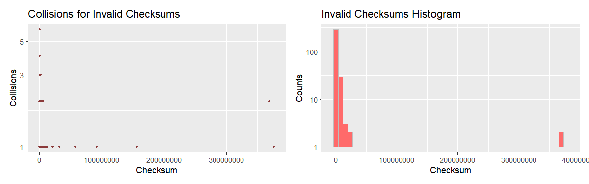
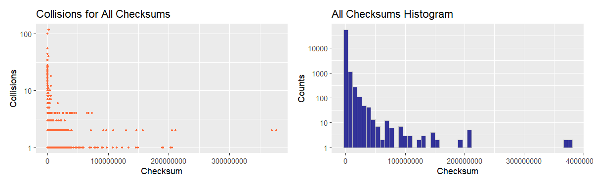
Take a look at the unscaled histogram plots.
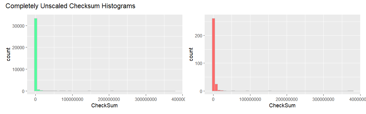
The CheckSum value range is quite large with most of the weight concentrated towards the smaller numbers. Concerns of similar nature pertain to the frequencies, where a few large values dominate the range. This is why here and there we log-scale the axes: sometimes x, sometimes y, other times both. Naturally, it has side-effects; when CheckSum is log-scaled, for example, the right distribution tail will seem shorter than it actually is.
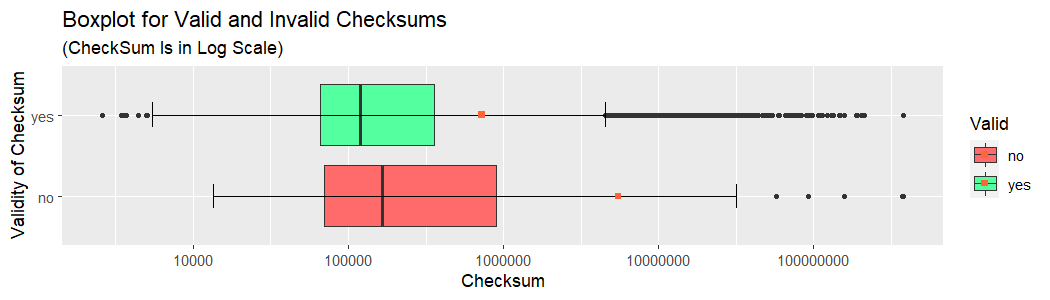
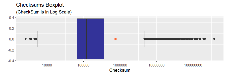
Both distributions are heavily skewed, with long right tails, but the invalid checksum distribution is noticeably more spread-out (as evidenced by a wider interquartile range) and shifted towards higher values (take a note of whiskers’ positions). Overall, checksum values tend to reside “on the smaller side”, the fact easily explained by the way they are computed. As a result, the distribution is far from uniform, which renders the checksum a less than perfect candidate for a hash of the PE file’s contents.
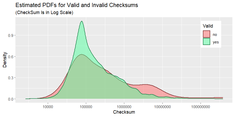
The density plots are even more informative in this respect.
Next we are going to look at distributions of valid and invalid checksums separately. After all, studying plots depicting various aspects of data and showing the same phnomena from multiple perspectives helps in developing stronger intuition about the nature of the data.
Distribution of Valid Checksums: A Detailed View
We begin with plots where the checksum is unscaled; they show how skewed the distribution actually is.
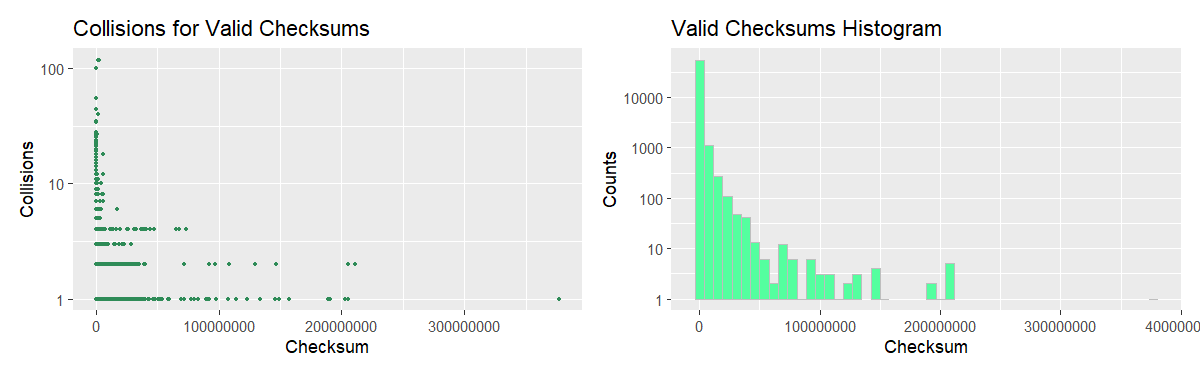
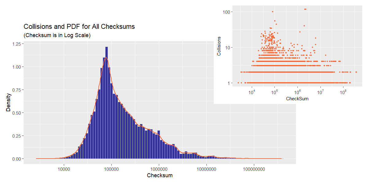
Keeping the figure above in mind, let us now plot the distribution in a more convenient form.
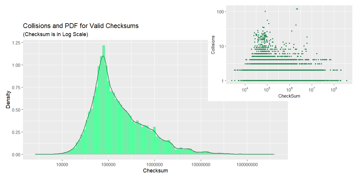
Considering the collision counts plot by itself, one would expect a bimodal PDF; however, the density plot assumes a different shape on account of the second “would-be-peak” being outweighed by lower values “from the same bin”. Here, the relatively narrow peak we predicted earlier is clearly visible, while the long thin tail is less so on account of its length having been concealed by logarithmic scale. Such a PDF shape implies that the probabiity of a random checksum value falling in the tight region around 105 is significantly higher as compared to the rest of the range.
Distribution of Invalid Checksums: A Detailed View
Following the scheme set up in the previous section, the plots for the incorrect checksums are constructed.
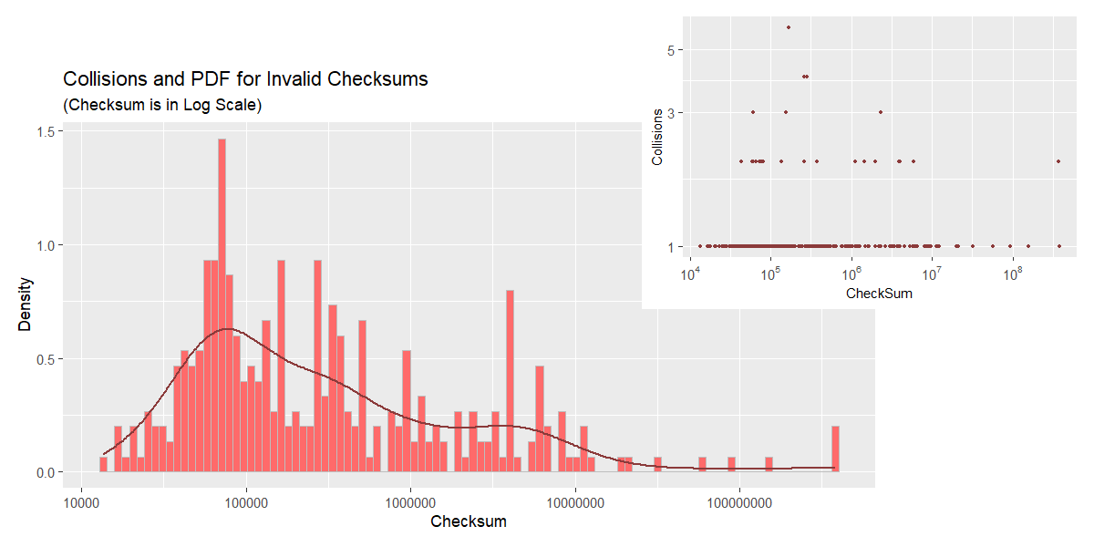
At first glance, collision counts plot looks very similar to that for valid checksums, but the histogram and KDE show a different picture. The estimated PDF is much flatter giving a decent probability of occuring to a wider range of values. Keep in mind, however, that there are significantly fewer binaries with incorrect non-zero checksum in the dataset, which makes one wonder if the sample in question can be deemed representative and what the plot would look like were we to obtain more data.
1
2
## Number of binaries with non-zero invalid checksum: 334.
## Number of binaries with valid checksum: 56652.
Combined Distribution of Valid and Valid Checksums: A Detailed View
For the sake of completeness, I am including the plots related to a combined distribution, the distribution all the CheckSum values in the dataset are drawn from, irrespective of their validity. Due to imbalance in the data, the combined checksum quantity is dominated by its valid constituent and, therefore, the plots should bring no surprises (neither should they require a commentary).
In order to obtain a dataframe containing both valid and invalid checksums, we perform an outer join on the CheckSum column with the subsequent summation of collision counts.
1
2
3
4
5
6
7
8
9
10
11
12
dfm <- merge(gdf[, c("CheckSum", "Collision_Count")],
             bdf[bdf$CheckSum > 0, c("CheckSum", "Collision_Count")],
             by = "CheckSum", all = TRUE)

names(dfm) <- c("CheckSum", "Collision_Count_Good", "Collision_Count_Bad")

dfm$Collision_Count_Good[is.na(dfm$Collision_Count_Good)] <- 0
dfm$Collision_Count_Bad[is.na(dfm$Collision_Count_Bad)] <- 0
dfm$Collision_Count <- dfm$Collision_Count_Good + dfm$Collision_Count_Bad

dfme <- data.frame(expand_column(dfm, "CheckSum", "Collision_Count"))
names(dfme) <- c("CheckSum")
Comparing to Checksums from Benign and Malicious PE Files Dataset
What have we discovered so far? For legitimate software, the valid/invalid checksum ratio turned out to be very close to that given in Michael Lester’ blog post. We also found out that vallid and invalid checksums were distributed differently, the latter suggesting that incorrect checkusms, being slightly different in nature, could not have appeared as a result of binary patching only (there is something else at play).
We have accomplished what we set out to do, but let us not call it a day yet. Would it not be interesting to see if the phenomenon that makes the distributions different has an even more prominent effect in malware? It might help with malware detection. The first idea that comes to mind is running the stats-collecting utility against a malware database. Logical as it is, this approach will not do since I would like the experiment to be easily reproducible by people of all backgrounds and not everyone has access to malware collections. There is another way. Notice that we do not actually need the binaries themselves: a dataset containing values stored in their PE headers will suffice, and I know of just the dataset we need (plus, some experience working with the dataset may come in handy).
We will use Mauricio Jara’s Benign and Malicious PE Files dataset, a collection of values (and a few derivatives thereof useful for malware detection) extracted from headers of PE files. The data was obtained by parsing binaries found in two Windows installations and an assortment of malware requested from VirusShare. Among the parsed PE fields is CheckSum and this is the only field we are going to use. That is, for every binary, we are given a checksum value (as stored in its PE header) and whether this module is malicious or benign (clean). Unfortunately, it is unknown if the given checkum is valid or not.
On a brighter note, unlike in the dataset created by our utility, even if we consider positive checksums only, there are enough datapoints of both kinds to avoid bias towards an over-represented class (in the context of our problem, at least).
1
2
3
4
5
mal_df <- read.csv("dataset_malwares.csv", header = TRUE, sep = ',')
cat(paste("Number of clean binaries with non-zero checksum",
          dim(mal_df[mal_df$CheckSum > 0 & mal_df$Malware == 0, ])[1]))
cat(paste("Number of malware binaries with non-zero checksum",
          dim(mal_df[mal_df$CheckSum > 0 & mal_df$Malware == 1, ])[1]))
1
2
## "Number of clean binaries with non-zero checksum 4889"
## "Number of malware binaries with non-zero checksum 9828"
First and foremost, let us check if the maximum value of CheckSum is the same as the one encountered previously.
1
summary(mal_df$CheckSum)
1
2
##       Min.    1st Qu.     Median       Mean    3rd Qu.       Max.
##          0       4476     205533  115491079     701512 4294967295
Alas! It is not. As it has already been mentioned, it is by coincidence that 0x167CF38F happens to be the maximum value in both, valid and invalid, checksum sets.
Let us take a look at the distribution of checksums in this dataset.
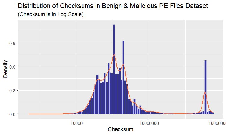
The plot is unlike anything we have seen up to this point. Why not dissect the distribution for the purpose of understanding it better? The way to go about it is to examine clean and malicious binaries separately. Let us begin with benign software.
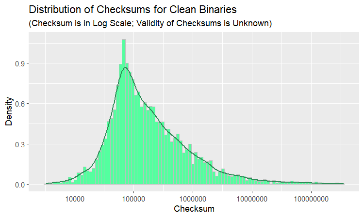
Either all green plots look alike or there is a definite similarity between distributions of correct checksums and checksums stored in the PE headers of clean binaries. Plotting them side by side should show if the similarity is real or imagined. To this end, putting apples and oranges in one basket, we combine binaries with correct checksum from the data collected by our utility and clean software from the Mauricio Jara’s dataset in a single dataframe.
1
2
3
4
5
6
7
8
9
10
11
12
13
14
15
16
17
#Malware and Benign PE Dataset
benign_df <- mal_df[mal_df$CheckSum > 0 & mal_df$Malware == 0,
                    c("CheckSum", "Malware")]
names(benign_df) <- c("CheckSum", "Type") #rename Malware (always 0) to Type

#valid checksums generated by our utility
egdf_t <- cbind(egdf, rep(1, length(egdf))) #assign all the datapoints Type 1
names(egdf_t) <- c("CheckSum", "Type")

#merge
apor_df <- rbind(benign_df, egdf_t)

factorize_type <- function(type) {
    factor(type, levels = c(0, 1), labels = c("Clean", "Valid Checksum"))
}

apor_df$Type <- factorize_type(apor_df$Type)
Voilà!
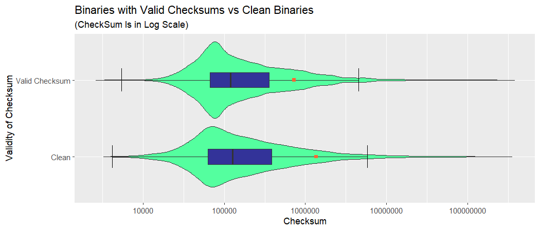
The resemblance is uncanny, as they say. It is especially remarkable given that the datasets were created nearly five years apart and come from completely different systems. Here are a few points of interest:
- Interquartile ranges and medians are almost identical, that is, 50% of data lies roughly in the same bounds.
- Beyond 1st and 3rd quantiles, the distribution for clean binaries is a little more spread-out; in particular, the distance between mean and median is greater and whiskers are situated farther apart.
- The following pertains to both distributions. The distributions are heavily skewed with very long right tails. Consequently, the mode and median are located relatively far apart. The median and mean, the latter influenced by the multitude and remoteness of outliers, are placed at even greater distance away from each other.
In this light, a distribution of Malware checksums is of particular interest and here it is:
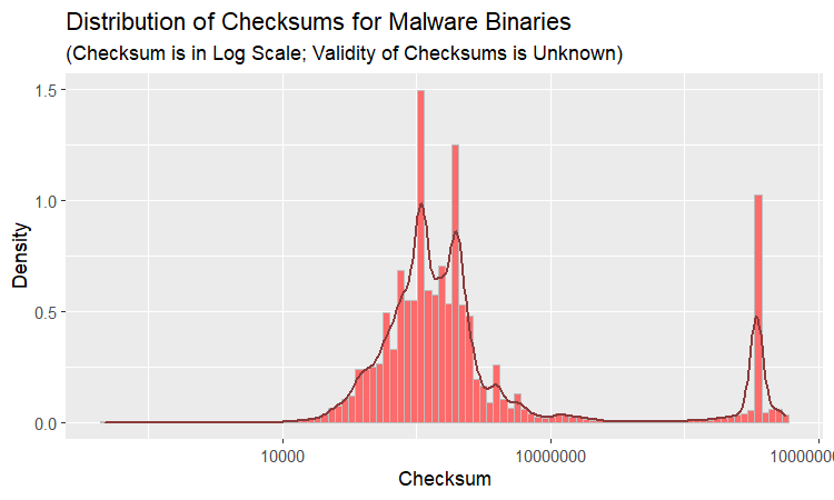
We can see that most of “irregularities”, that set the distribution of checksums in this dataset apart, come from the malicious modules and it stands to reason that malware binaries are more likely to have incorrect checksums. Recall, that, according to Michael Lester, an absolute majority of clean binaries have correct checksums; it is malware (83% of malicious modules!) that supplies us with unusual checksum values and this experiment may serve as an illustration of this statement.
The origin of incorrect checksums would be an interesting topic to explore: were it simply the matter of packers forgetting to update the PE headers, the distribution would be the same as for valid checksums. Yet, the PDF looks different and, as predicted, we see more of these differences in malicious modules.
The Checksum Algorithm
What is so peculiar about formation of invalid checksums that affects their distribution in such a manner, I cannot tell you (it is a topic for another study), but, at least, I can explain why valid checksums are distributed the way they are.
File checksum (PE files are no exception) is supposed to help discover corrupted files and, as such, is usually designed to detect even the slightests (e.g., 1-bit-long) changes in file’s contents. In this regard, checksum can be considered a hash function of the file’s contents since, ideally, different byte sequences should result in different checksums. The hash function that achieves it most effectively follows a uniform distribution. Valid checkssums, however, are spread rather unevenly along the range of 32-bit integers. What is going on? The answer lies in the algorithm that computes PE checksums.
Where can one find the checksum algorithm Windows uses? Why, in the code of Microsoft’s own CheckSumMappedFile() utilized by our stats-collecting utility. Straight to the primary source! CheckSumMappedFile(), in turn, calls the ChkSum() subroutine that computes the checksum. I went ahead and used a debugger to generate the assembly listings (64-bit) for this function. Let us take a look.
I am skipping all the ducking and diving involved in ensuring the function works correctly with data of various sizes and alingments and including only the “heavy-lifting” chunk where the bulk of computation takes place.
1
2
3
4
5
6
7
8
9
10
11
12
13
14
15
16
17
18
19
20
21
22
23
24
25
26
27
28
29
30
31
32
33
34
35
36
37
38
39
40
ChkSum:
;[...]
ChkSum+0ECh:
add         eax,dword ptr [rdx]
adc         eax,dword ptr [rdx+4]
adc         eax,dword ptr [rdx+8]
adc         eax,dword ptr [rdx+0Ch]
adc         eax,dword ptr [rdx+10h]
adc         eax,dword ptr [rdx+14h]
adc         eax,dword ptr [rdx+18h]
adc         eax,dword ptr [rdx+1Ch]
adc         eax,dword ptr [rdx+20h]
adc         eax,dword ptr [rdx+24h]
adc         eax,dword ptr [rdx+28h]
adc         eax,dword ptr [rdx+2Ch]
adc         eax,dword ptr [rdx+30h]
adc         eax,dword ptr [rdx+34h]
adc         eax,dword ptr [rdx+38h]
adc         eax,dword ptr [rdx+3Ch]
adc         eax,dword ptr [rdx+40h]
adc         eax,dword ptr [rdx+44h]
adc         eax,dword ptr [rdx+48h]
adc         eax,dword ptr [rdx+4Ch]
adc         eax,dword ptr [rdx+50h]
adc         eax,dword ptr [rdx+54h]
adc         eax,dword ptr [rdx+58h]
adc         eax,dword ptr [rdx+5Ch]
adc         eax,dword ptr [rdx+60h]
adc         eax,dword ptr [rdx+64h]
adc         eax,dword ptr [rdx+68h]
adc         eax,dword ptr [rdx+6Ch]
adc         eax,dword ptr [rdx+70h]
adc         eax,dword ptr [rdx+74h]
adc         eax,dword ptr [rdx+78h]
adc         eax,dword ptr [rdx+7Ch]
adc         eax,0
add         rdx,80h
sub         ecx,80h
jne         ChkSum+0ECh
;[...]
NOTE: Before us is an example of loop unrolling, an optimization technique aiming to speed up loops. It consists in extending loop’s body over multiple iterations in order to save on condition checks and, sometimes, counter increments.
For example, unrolling the loop for (int i = 0; i < n; i++) do_work(i); over 3 iteration would result in something along the lines of
for (int i = 0; i < 3*(n/3); i += 3) {
    do_work(i);
    do_work(i + 1);
    do_work(i + 2);
}

if (n % 3 > 0) {
    do_work(n - (n % 3));
    if (n % 3 > 1)
        do_work(n - (n % 3) + 1);
}
Thus, the number of times the loop condition is tested would decrease by a factor of 3.
As is, this solution looks rather ugly and I strongly encourage everyone who has not done so already to check out Duff’s device for a much more elegant implementation of loop unrolling.
No course on compilers goes without (at the very least) mentioning this technique; here, we are given a chance to “observe it in the wild”.
Implemented in this assembly snippet is a loop that sums up all the dwords in an array, unrolled over 32 iterations. Notice that the summation is performed with carry, i.e. sum += data[i] + CF or, in other words, if sum + data[i] does not fit in a dword and overflows, an additional bit will be added at the next iteration: sum += data[i+1] + 1.
So far, the code has seemed reasonable enough; the inexplicable part comes next. Shortly before it returns, the function does the following:
1
2
3
4
5
6
7
8
mov         edx,eax
shr         edx,10h
and         eax,0FFFFh
add         eax,edx
mov         edx,eax
shr         edx,10h
add         eax,edx
and         eax,0FFFFh
The sum (stored in eax) folds in itself: the higher 16-bit word, shifted right by 16 bits, is summed with the lower word. The operation is performed two times in order to ensure that the result fits into 16 bits (then, at the very end, the size of pe file is added, but on that – later).
While this interpretation matches the implementation found in pefile and Michael Lester’s blog post, it leaves one in a state of mild confusion. Why would one reduce a perfectly good 32-bit value to as little as 16 bits? The developer of php-winpefile at CubicleSoft (whose name I deduced to be Thomas Hruska, but I might be mistaken) shares the sentiment:
Win16 NE header checksum calculation. Knowledge of how to calculate this was difficult to come by. […] Want to know what’s harder to find than Win16 NE header checksum calculation logic? Finding sane Win32 PE header checksum calculation logic.
In the end, it was php-winpefile’s source code where I finally found the explanation: the original algorithm (chosen, as I suspect, for historical reasons) sums 16- (and not 32-) bit values; what we often come across is yet another optimization, the outcome of it being half as many reads and additions as well as 32-bit-aligned addresses (though caching makes these estimates somewhat irrelevant). php-winpefile contains an unoptimzed implementation of the algorithm in php, which can be found here. I have written my own version, in C, and am presenting it (below) for the reader’s perusing pleasure.
1
2
3
4
5
6
7
8
9
10
11
12
13
14
15
16
17
18
19
20
21
22
23
24
25
26
27
28
29
30
31
32
33
34
35
36
37
38
39
40
41
42
43
DWORD ComputeCheckSumUnoptimized(PVOID pMap, DWORD dwFileSize)
{
    IMAGE_DOS_HEADER* pDosHdr = (IMAGE_DOS_HEADER*)pMap;
    IMAGE_NT_HEADERS* pHdr = (IMAGE_NT_HEADERS*)((BYTE*)pMap + pDosHdr->e_lfanew);

    //Done in the interest of the code being fundamentally correct
    //(the offset is actually the same)
    DWORD dwCheckSumOffset = offsetof(IMAGE_NT_HEADERS, OptionalHeader) +
        (pHdr->OptionalHeader.Magic == IMAGE_NT_OPTIONAL_HDR32_MAGIC ?
        offsetof(IMAGE_OPTIONAL_HEADER32, CheckSum) :
        offsetof(IMAGE_OPTIONAL_HEADER64, CheckSum));

    uint16_t* pwChecksum = (uint16_t*)((BYTE*)pHdr + dwCheckSumOffset);

    DWORD dwSize = dwFileSize;
    uint16_t* pBase = (uint16_t*)(pMap); //16-bit!
    uint16_t wSum = 0;
    uint8_t bCarry = 0;

    while (dwSize >= sizeof(uint16_t)) {

        //Skipping the CheckSum Field
        if (pBase == pwChecksum) {
            pBase += 2;
            dwSize -= sizeof(uint32_t);
            continue;
        }

        dwSize -= sizeof(uint16_t);

        bCarry = _addcarry_u16(bCarry, wSum, *pBase++, &wSum);
    }

    if (dwSize != 0) {
        //the last byte, when the size of the file is not a multiple of two
        bCarry = _addcarry_u16(bCarry, wSum, *(BYTE*)pBase, &wSum);
    }

    //add a possible carry bit
    _addcarry_u16(bCarry, wSum, 0, &wSum);

    return wSum + dwFileSize;
}
Naturally, this implementation is for the purpose of illustration only and not meant to be used in practice. The code should be self-explanatory; _addcarry_u16, a MS VC’s intrinsic function, translates directly to an adc instruction; for clarity, fixed-width types are used (where it is helpful). Notice, that in the final line, the file size passed as an argument is added to the 16-bit sum and the result is returned as the checksum.
Now that the mystery of a folding-in sum has been solved, let us move to the second element of the puzzle – file size.
From experience, executable files are typically small, with the sizes measured in kilobytes; a back-of-the-envelope script-in-a-temp-folder computation will further convince us in the validity of this estimation. I will save you half-an-hour of coding; here is a simple python script that collects file sizes-relate statistics.
1
2
3
4
5
6
7
8
9
10
11
12
13
14
15
16
17
18
19
20
21
22
23
24
25
26
27
28
29
30
31
32
33
34
35
36
37
38
39
40
41
42
43
44
45
46
47
import os
import sys
import struct

def check_pe_magic_numbers(path, size):
    """Checks magic numbers indicating that the file is a PE binary"""
    s = struct.Struct("<H58xI")
    if size < s.size:
        return False;

    with open(path, "rb") as fl:
        ps = s.unpack(fl.read(s.size))
        if ps[0] != 0x5A4D or size < ps[1] + 2:
            return False
        fl.seek(ps[1], 0)
        return fl.read(1) == b'P' and fl.read(1) == b'E'


def main(args):
    if len(args) < 3:
        print("usage: ", args[0], "<root dir> <out csv>")
        return;

    sizes = {}
    for root, dirs, files in os.walk(args[1]):
        fls = [ f for f in files if f.lower().endswith((".dll", ".exe", ".sys")) ]
        for f in fls:
            try:
                path = os.path.join(root, f)
                fsz = os.path.getsize(path)

                if not check_pe_magic_numbers(path, fsz):
                    continue

                if not fsz in sizes:
                    sizes[fsz] = 0
                    sizes[fsz] += 1

            except Exception as e:
                print("Error accessing", path, "(", str(e), ")")

        lns = [ str(sz) + " " + str(sizes[sz]) + "\n" for sz in sizes ]
        with open(args[2], "w") as fl:
            fl.writelines(lns)

if __name__ == "__main__":
    main(sys.argv)
check_pe_magic_numbers() requires an explanation. Running an early version of this script, I discovered quite a few specimen, which, in spite of .exe and .dll extensions, were not PE files at all, but something else: shell code, for example (not to mention .sys files, adopted by various facilities such as swapping and hibernation). check_pe_magic_numbers() ensures that all the counted files comply with the PE format.
Let us see what the stats look like.
1
2
3
4
5
6
7
8
9
10
11
12
import matplotlib.pyplot as plt
%matplotlib inline
import pandas as pd
import numpy as np

data = pd.read_csv("out_sizes.csv", sep = " ",
                   names = ["size", "count"],
                   header = None)
data["SizeInKB"] = data["size"] / 1024
data = data.loc[data.index.repeat(data["count"]), "SizeInKB"].reset_index(drop = True)
data.plot(kind = "hist", bins = 5000, logx = True,
          title = "Histogram for Binary Sizes (in Kilobytes)")
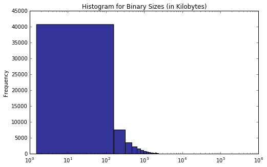
As expected, the absolute majority of PE files are well under 1 MB in size. With most of the file sizes lying in the range from 0xFFF to 0xFFFFF and the contents digest limited to 16 bits (0xFFFF), the resulting checksum values rarely have the highest byte set to anything other than zero (or fall below 0xFFF). This fact should explain why the (estimated) PDF of the valid checksum distribution has the shape it does.
On Invalid Checksums
The case of valid checksums was fairly straightforward and, I am afraid, the account of uncovering their “nature” will not make it into the bestsellers list; invalid checksums, particularly non-zero ones, on the other hand, are much more mysterious. It so happens, there are many reasons why a checksum may end up invalid and tracking down the story behind each and every one of them is an investigation in its own right. Unfortunately, we are running out of space-time, but, nevertheless, the statistics collected by our utility may offer some insights into the subject.
Let us run summary() against the csv containing data on bad non-zero checksums.
1
2
3
4
5
6
7
8
                signature            rich
(bad digest)         :  3   No Rich    :162
(no signature)       :228   Rich Header:172
Google Inc           :  5
Google LLC           :  3
Microsoft Corporation: 88
Mozilla Corporation  :  1
Windows Phone        :  6
There were only 334 such binaries on my computer, not enough to reach any definite conclusions; besided, I chose to record two attributes only: Rich header presence and signature validity. That said, the data thus collected does shed a light, however dim, on the origin of checksum errors. Below are the meager titbits of information I managed to extract. Of the modules with non-zero invalid checksums:
- 51% contain Rich header, a distiguishing mark of Microsoft’s compiler products, meaning that the corresponding checksum errors were probably introduced by post-buid patching.
- 31% are signed (by well-known entities) and verified, strongly suggesting that their checksums did not result from malicious tampering.
- 94 (28%) were supplied by Microsoft itself, thereby confirming that checksum correctness is generally not regarded as important.
The thing immediately becoming a source of anxiety is the record of three signed files marked by a “bad digest” that, evidently, were patched after they had been signed. Surely, it is a clear indication of malicious intent. Two of these files, it turns out, come from the small collection of malformed binaries I tested my SEH-data-parsing extension for pefile on (so I was not completely correct in calling my system typical); they do not count. What about the third one? Well, I do not know for certain. It is the version of Qt5Core.dll included in one of R Studio installiations; I found numerous complains about the issue online, but have not made time for further investigation yet.
There is a third field, omitted in the listing above, in the bad checksums csv – full paths to the PE files. Having read through the list, I came across a few (11 out of 334, to be exact) files, all named “Uninstall.exe”. Interestinly, the corresponding setup files (used to install that software) have matching CheckSum values that are valid for the distributives but invalid for uninstall.exe. Apparently, files “uninstall.exe” are generated “on the fly” (this is why they are not signed) by the kind of installer all these software products utilize, and, in the process, the checksum value is simply copied from PE header of the setup executable. Below are the examples illustating the phenomenon.
| path | checksum | valid? | signed | |
| Ex. 1: | \SpeedFan\uninstall.exe | 0x300689 | no | (no signature) |
| \Downloads\instspeedfan452.exe | 0x300689 | yes | SOKNO S.R.L. | |
| Ex. 2: | \JetBrains\PyCharm\bin\Uninstall.exe | 0x167CF38F | no | (no signature) |
| \Downloads\pycharm-community-2021.3.2.exe | 0x167CF38F | yes | JetBrains s.r.o. |
By the way, did anyone notice that PyCharm’s checksum, 0x167CF38F, is the same as the maximum CheckSum value shared by both valid and invalid checksum sets? The entire PyCharm development environment, packed in a single fat distribution file, weights a ton, thereby producing a very large checksum value, which is then associated with two exe files, but only with to one of them – rightfully. There is nothing to it. Another mystery solved! One does begin feeling like a detective after a while…
Conclusion
By the way of conlusion, let me briefly summarize the findings presented in this post.
- Ratio of valid to invalid checksums computed for binaries of one typical system turned out to be very close to the same reported by Michael Lester at Practical Security Analytics. It may reflect popularity of certain development tools and their usage patterns.
- Comparing distributions of valid and invalid checksums from one dataset, and of checksums computed for clean and malicious binaries from another domonstrated that, while valid checksums and checksums of benign modules were nearly identically distributed, invalid checksums and malware modues were the main sources of differences, thereby confirming that malware is more likely to have incorrect checksums.
- Valid checksums values are spread unevently along the range of 32-bit integers; an explanation for this distribution shape lies in the algorithm that computes them.
- Digitally-signed software from well-known vendors is prone (of course, to a lesser degree) to checksum errors.
– Ry Auscitte
References
- Michael Lester, Threat Hunting with the PE Checksum, Practical Security Analytics (2019)
- Optional Header Windows-Specific Fields, PE Format, Microsoft Docs
- /RELEASE (Set the Checksum), MSVC Linker Options, MSVC Linker Reference
- Ero Carrera, pefile: a Python module to read and work with PE (Portable Executable) files
- Mauricio Jara, Benign and Malicious PE Files Dataset for Malware Detection, Kaggle
- CubicleSoft, php-winpefile, Windows PE File Tools for PHP